Recall: The Firm's Two Problems
1st Stage: firm's profit maximization problem:
Choose: < output >
In order to maximize: < profits >
2nd Stage: firm's cost minimization problem:
Choose: < inputs >
In order to minimize: < cost >
Subject to: < producing the optimal output >
- Minimizing costs ⟺ maximizing profits

A Competitive Market
- We assume (for now) the firm is in a competitive industry:
Firms’ products are perfect substitutes
Firms are “price-takers”, no one firm can affect the market price
Market entry and exit are free†
† Remember this feature. It turns out to be the most important feature that distinguishes different types of industries!
Profit
Recall that profit is: π=pq⏟revenues−(wl+rk)⏟costs
We’ll first take a closer look at costs today
Next class we’ll put costs together with revenues to find optimal q∗ that maximizes π (the first stage problem)

Production Costs are Opportunity Costs
- Remember, economic costs are broader thanthe common conception of “cost”
- Accounting cost: monetary cost
- Economic cost: value of next best alternative use of resources given up (i.e. opportunity cost)


Production Costs are Opportunity Costs
This leads to the difference between
- Accounting profit: revenues minus accounting costs
- Economic profit: revenues minus accounting & opportunity costs
A really difficult concept to think about!
Production Costs are Opportunity Costs
Another helpful perspective:
Accounting cost: what you historically paid for a resource
Economic cost: what you can currently get in the market for a selling a resource
- Resource's value in alternative uses
A Reminder: It's Demand all the Way Down!
Supply is actually Demand in disguise!
The (opportunity) cost producers must pay to purchase (scarce) inputs to produce products comes from the fact that other people demand those same inputs to consume or produce other things for other purposes!
- You are not paying the price just to buy them, but also to pull them out of other valuable lines of production in the economy!
Production Costs are Opportunity Costs
Because resources are scarce, and have rivalrous uses, how do we know we are using resources efficiently??
In functioning markets, the market price measures the opportunity cost of using a resource for an alternative use
Firms not only pay for direct use of a resource, but also indirectly compensate society for "pulling the resource out" of alternate uses in the economy!
Production Costs are Opportunity Costs
- Every choice incurs an opportunity cost
Examples:
- If you start a business, you may give up your salary at your current job
- If you invest in a factory, you give up other investment opportunities
- If you use an office building you own, you cannot rent it to other people
- If you hire a skilled worker, you must pay them a high enough salary to deter them from working for other firms
Opportunity Cost is Hard for People

Opportunity Costs vs. Sunk Costs
Opportunity cost is a forward-looking concept
Choices made in the past with non-recoverable costs are called sunk costs
Sunk costs should not enter into future decisions
Many people have difficulty letting go of unchangeable past decisions: sunk cost fallacy

Sunk Costs: Examples

Sunk Costs: Examples

Sunks Costs: Examples

Common Sunk Costs in Business
Licensing fees, long-term lease contracts
Specific capital (with no alternative use): uniforms, menus, signs
Research & Development spending
Advertising spending
The Accounting vs. Economic Point of View I
- Helpful to consider two points of view:
“Accounting point of view”: are you taking in more cash than you are spending?
“Economic point of view”: is your product you making the best social use of your resources
- i.e. are there higher-valued uses of your resources you are keeping them out of?
The Accounting vs. Economic Point of View II
Implications for society: are consumers best off with you using scarce resources (with alternative uses!) to produce your current product?
Remember: this is an economics course, not a business course!
- Economists are pro-market, not pro-business!
- What might be good/bad for one business might have bad/good consequences for society!
Fixed vs. Variable costs: Examples

Example: Airlines
Fixed costs: the aircraft
Variable costs: getting one more customer in a seat
Fixed vs. Variable costs: Examples
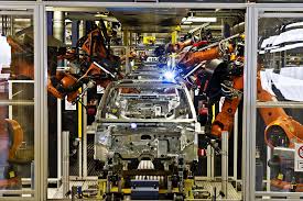
Example: Car Factory
Fixed costs: the factory, machines in the factory
Variable costs: producing one more car
Fixed vs. Variable costs: Examples
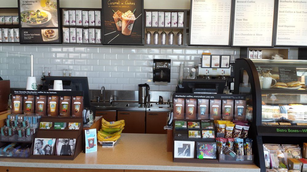
Example: Starbucks
Fixed costs: the retail space
Variable costs: selling one more cup of coffee
Fixed vs. Sunk costs
Diff. between fixed vs. sunk costs?
Sunk costs are a type of fixed cost that are not avoidable or recoverable
Many fixed costs can be avoided or changed in the long run
Common fixed, but not sunk, costs:
- rent for office space, durable equipment, operating permits (that are renewed)
When deciding to stay in business, fixed costs matter, sunk costs do not!
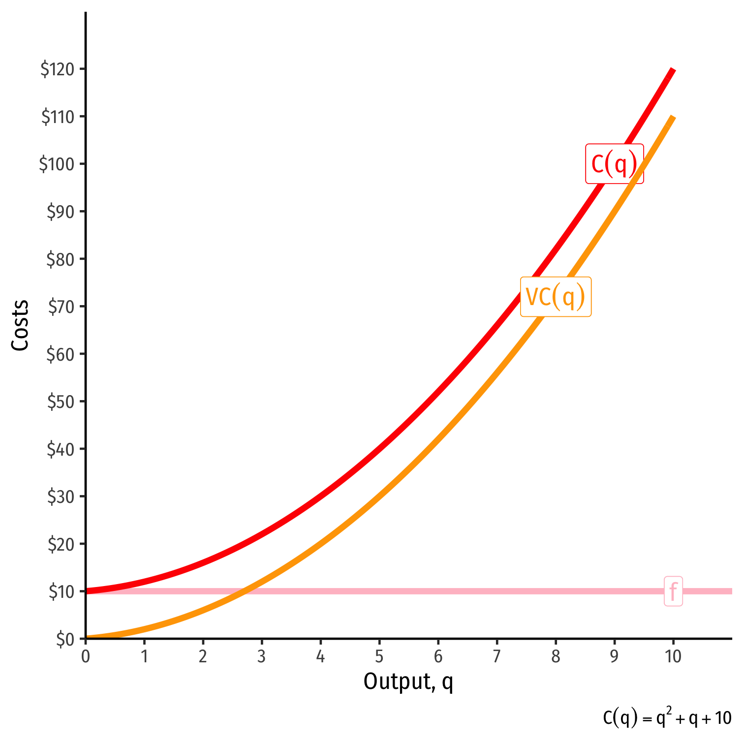
Cost Functions: Example, Visualized
| q | f | VC(q) | C(q) |
|---|---|---|---|
| 0 | 10 | 0 | 10 |
| 1 | 10 | 2 | 12 |
| 2 | 10 | 6 | 16 |
| 3 | 10 | 12 | 22 |
| 4 | 10 | 20 | 30 |
| 5 | 10 | 30 | 40 |
| 6 | 10 | 42 | 52 |
| 7 | 10 | 56 | 66 |
| 8 | 10 | 72 | 82 |
| 9 | 10 | 90 | 100 |
| 10 | 10 | 110 | 120 |
The Importance of Marginal Cost
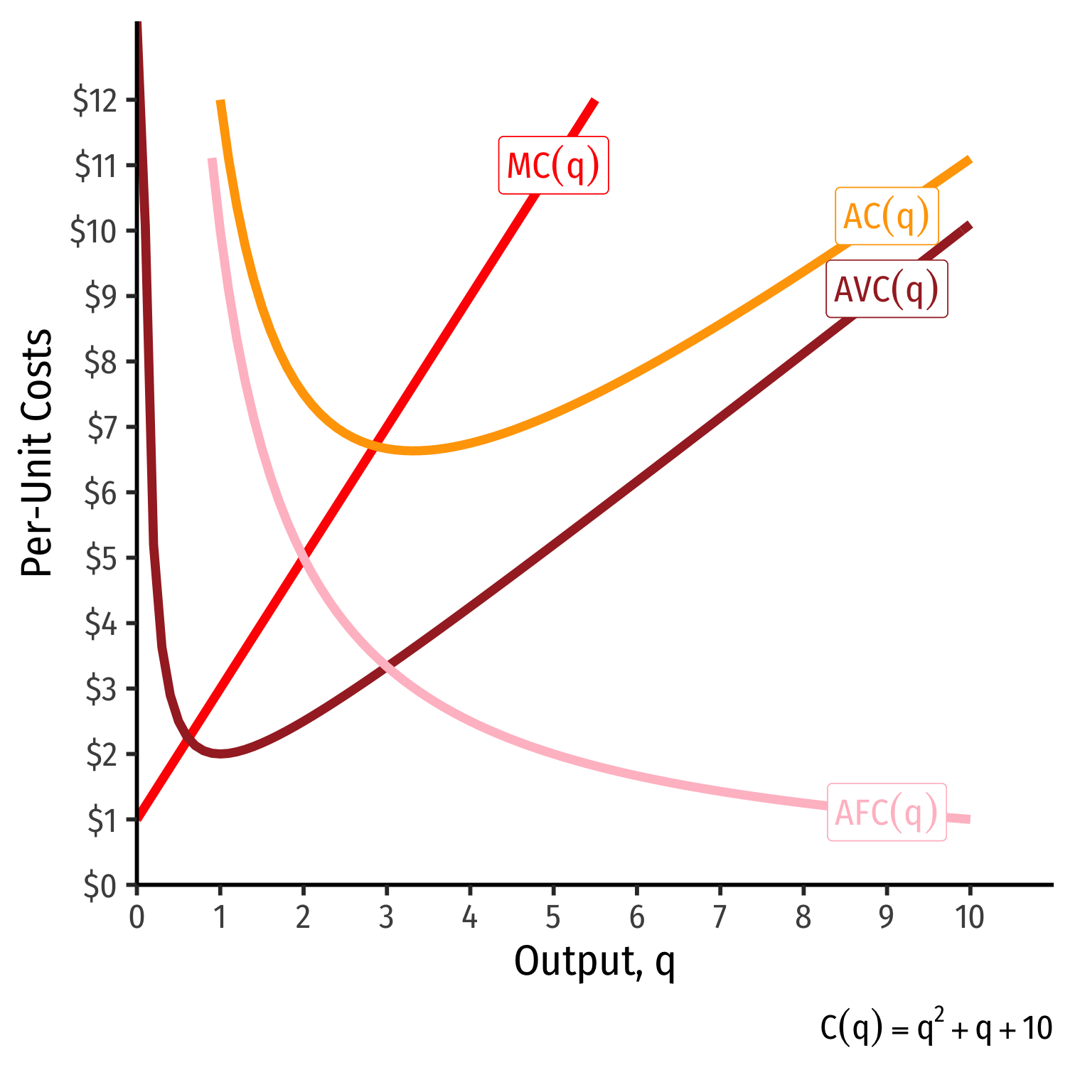
Average and Marginal Costs: Visualized
| q | C(q) | MC(q) | AFC(q) | AVC(q) | AC(q) |
|---|---|---|---|---|---|
| 0 | 10 | − | − | − | − |
| 1 | 12 | 2 | 10.00 | 2 | 12.00 |
| 2 | 16 | 4 | 5.00 | 3 | 8.00 |
| 3 | 22 | 6 | 3.33 | 4 | 7.30 |
| 4 | 30 | 8 | 2.50 | 5 | 7.50 |
| 5 | 40 | 10 | 2.00 | 6 | 8.00 |
| 6 | 52 | 12 | 1.67 | 7 | 8.70 |
| 7 | 66 | 14 | 1.43 | 8 | 9.40 |
| 8 | 82 | 16 | 1.25 | 9 | 10.25 |
| 9 | 100 | 18 | 1.11 | 10 | 11.10 |
| 10 | 120 | 20 | 1.00 | 11 | 12.00 |
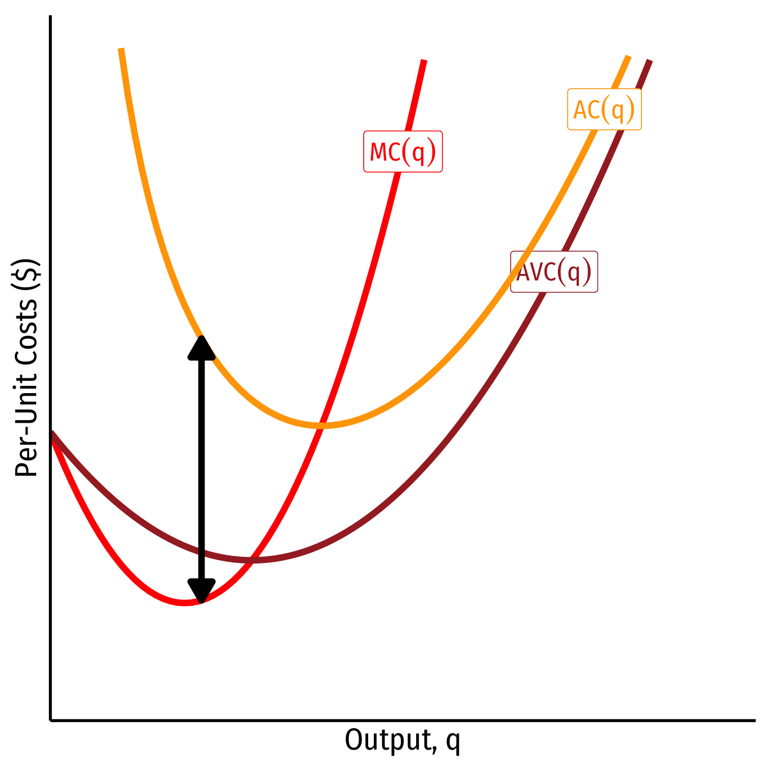
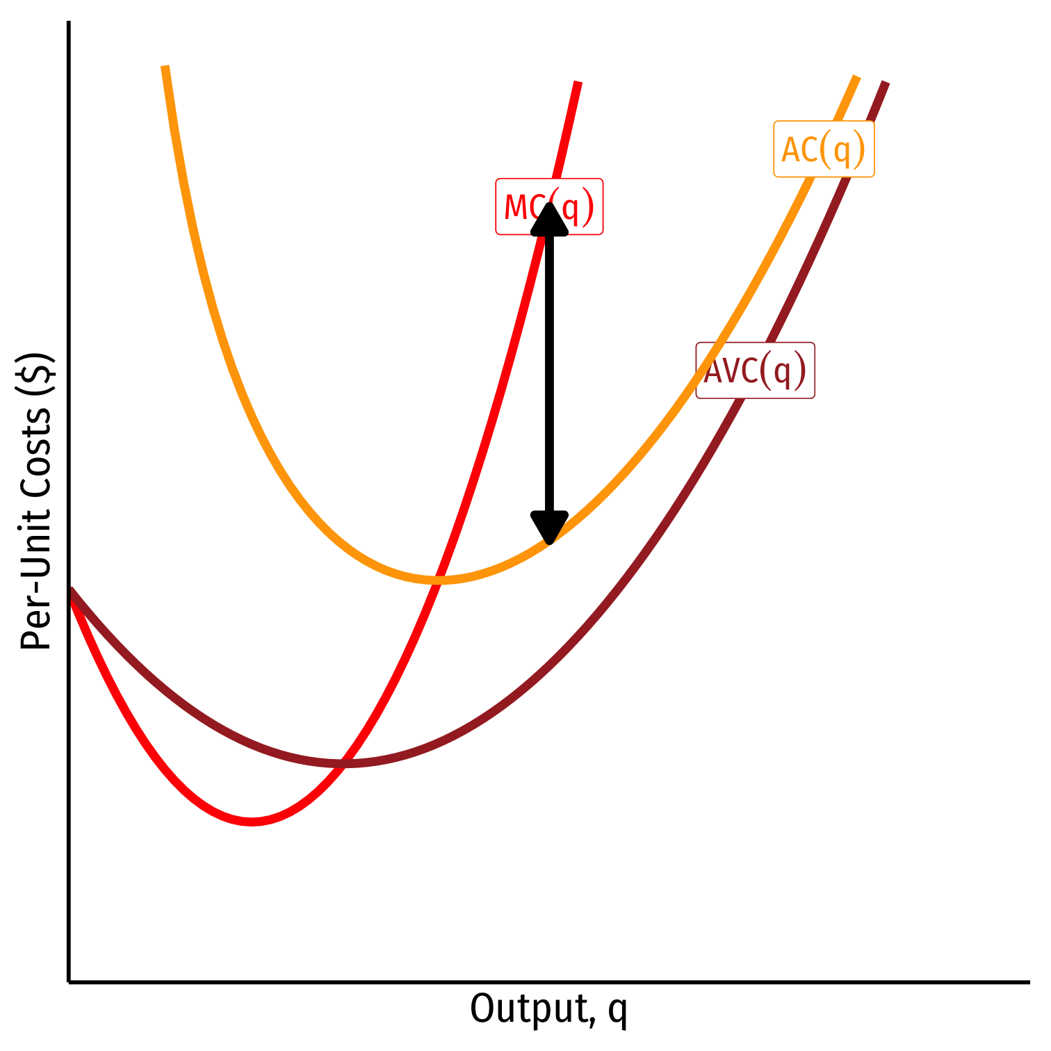
Relationship Between Marginal and Average
Mathematical relationship between a marginal & an average value
If marginal < average, then average ↓
Relationship Between Marginal and Average
Mathematical relationship between a marginal & an average value
If marginal < average, then average ↓
If marginal > average, then average ↑
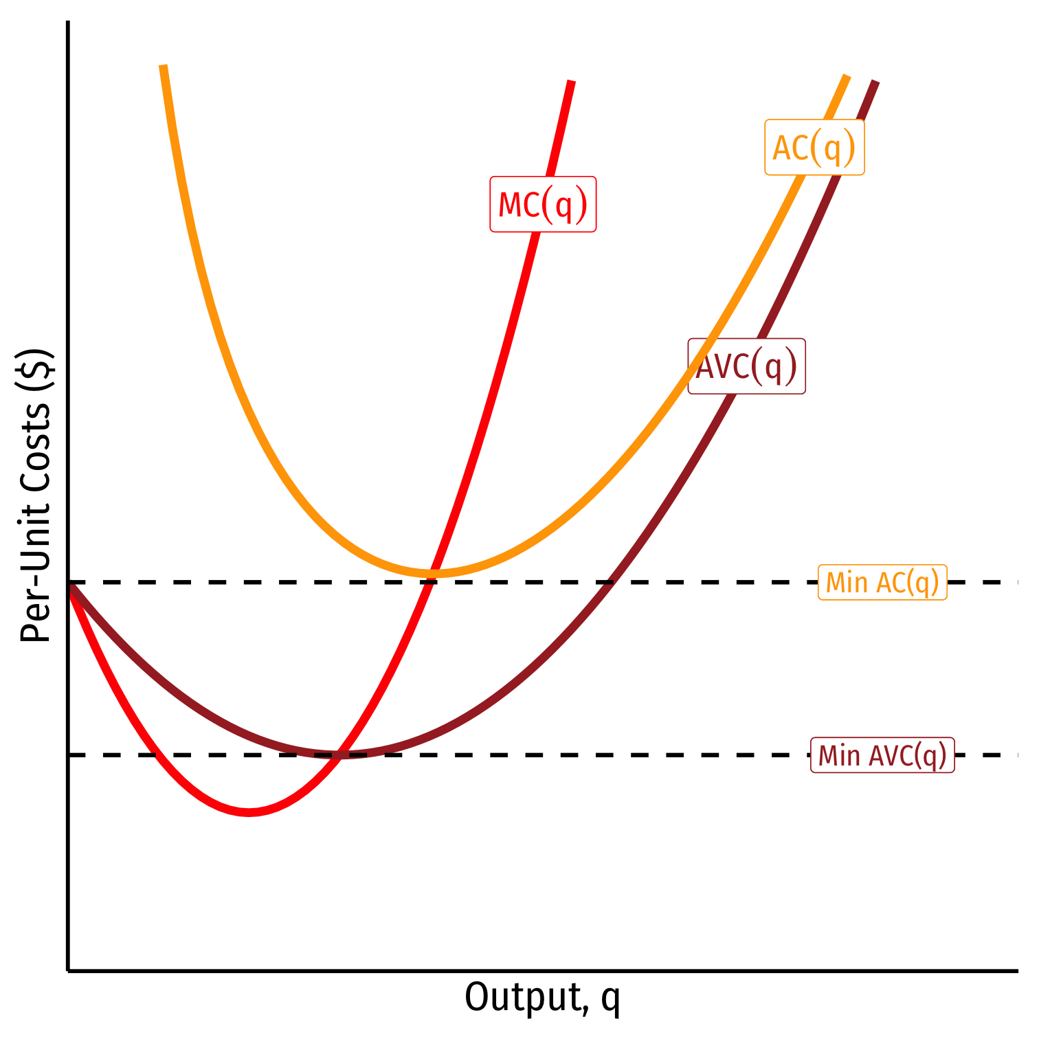
Relationship Between Marginal and Average
Mathematical relationship between a marginal & an average value
If marginal < average, then average ↓
If marginal > average, then average ↑
When marginal = average, average is maximized/minimized
- When MC=AC, AC is at a minimum
When MC=AVC, AVC is at a minimum
Economic importance (later): Break-even price & shut-down price
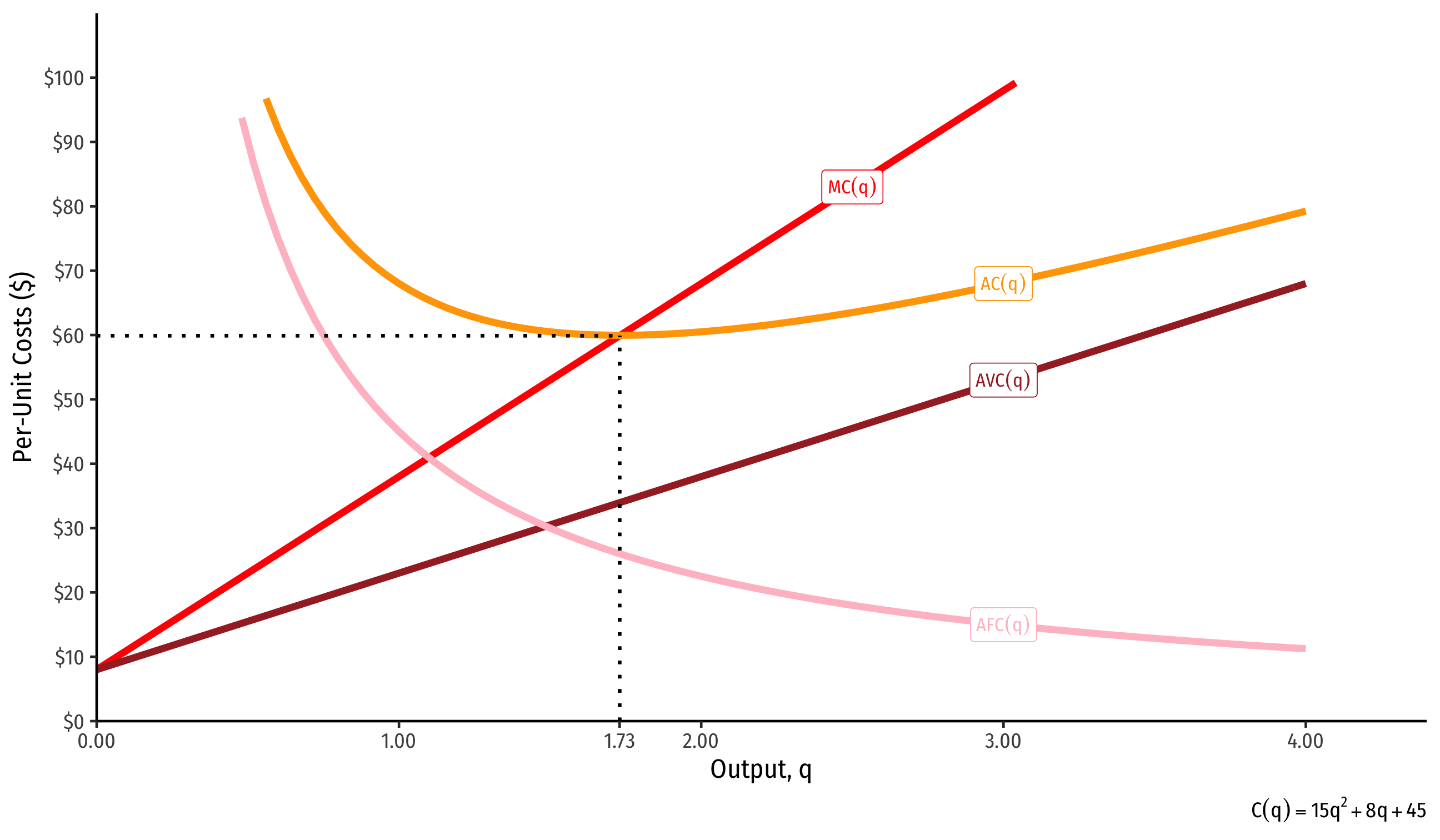
Costs: Example: Visualized
Costs in the Long Run
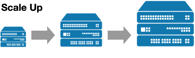
Long run: firm can change all factors of production & vary scale of production
Long run average cost, LRAC(q): cost per unit of output when the firm can change both l and k to make more q
Long run marginal cost, LRMC(q): change in long run total cost as the firm produce an additional unit of q (by changing both l and/or k)

Average Cost in the Long Run
Long run: firm can choose k (factories, locations, etc)
Separate short run average cost (SRAC) curves for each amount of k potentially chosen
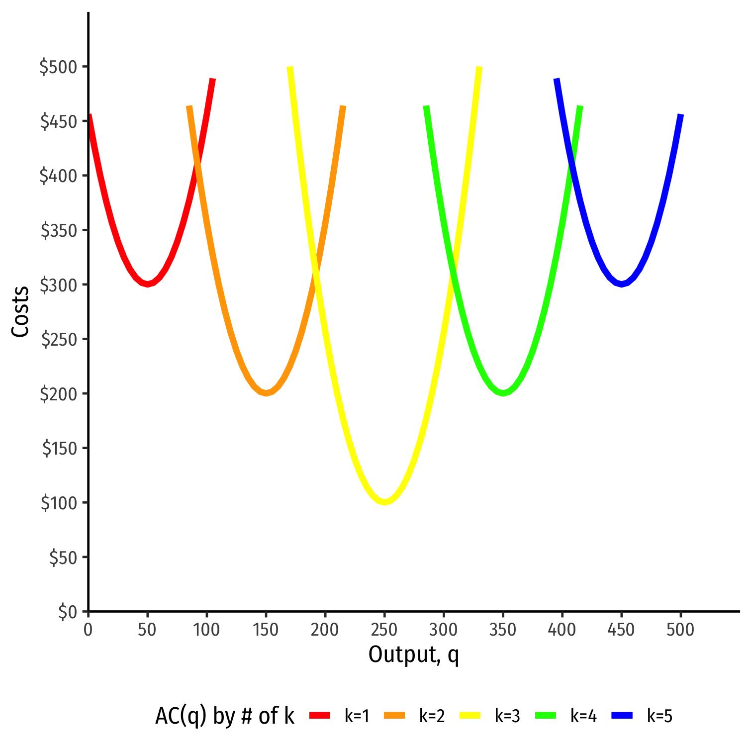
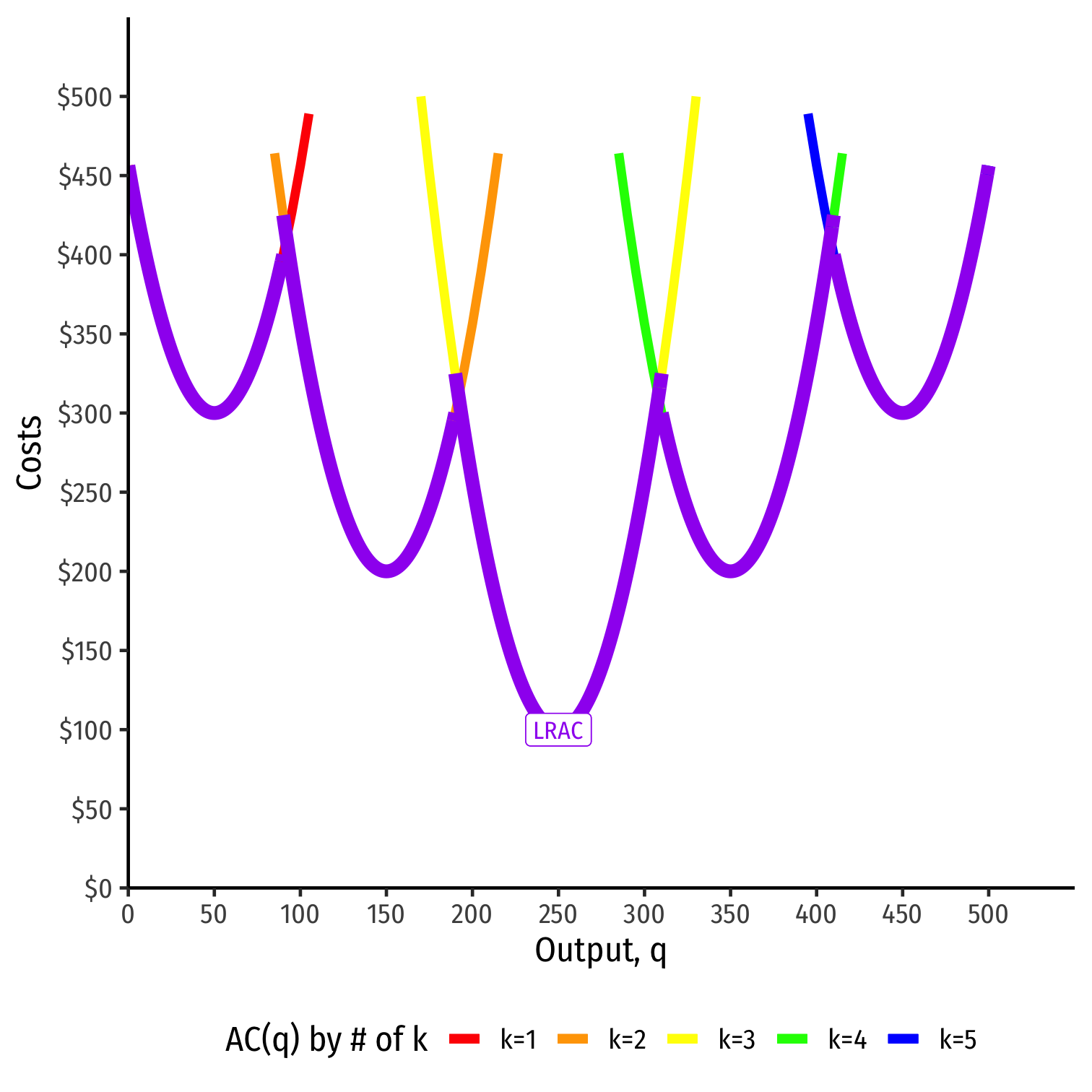
Average Cost in the Long Run
Long run: firm can choose k (factories, locations, etc)
Separate short run average cost (SRAC) curves for each amount of k potentially chosen
Long run average cost (LRAC) curve "envelopes" the lowest (optimal) parts of all the SRAC curves!
"Subject to producing the optimal amount of output, choose l and k to minimize cost"
Long Run Costs & Scale Economies I
Further important properties about costs based on scale economies of production: change in average costs when output is increased (scaled)
Economies of scale: average costs fall with more output
- High fixed costs AFC>AVC(q) low variable costs
Diseconomies of scale: average costs rise with more output
- Low fixed costs AFC<AVC(q) high variable costs
Constant economies of scale: average costs don’t change with more output
- Firm at minimum average cost (optimal plant size), called minimum efficient scale (MES)
Long Run Costs & Scale Economies I
Note economies of scale ≠ returns to scale!
Returns to Scale (last class): a technological relationship between inputs & output
Economies of Scale (this class): an economic relationship between output and average costs
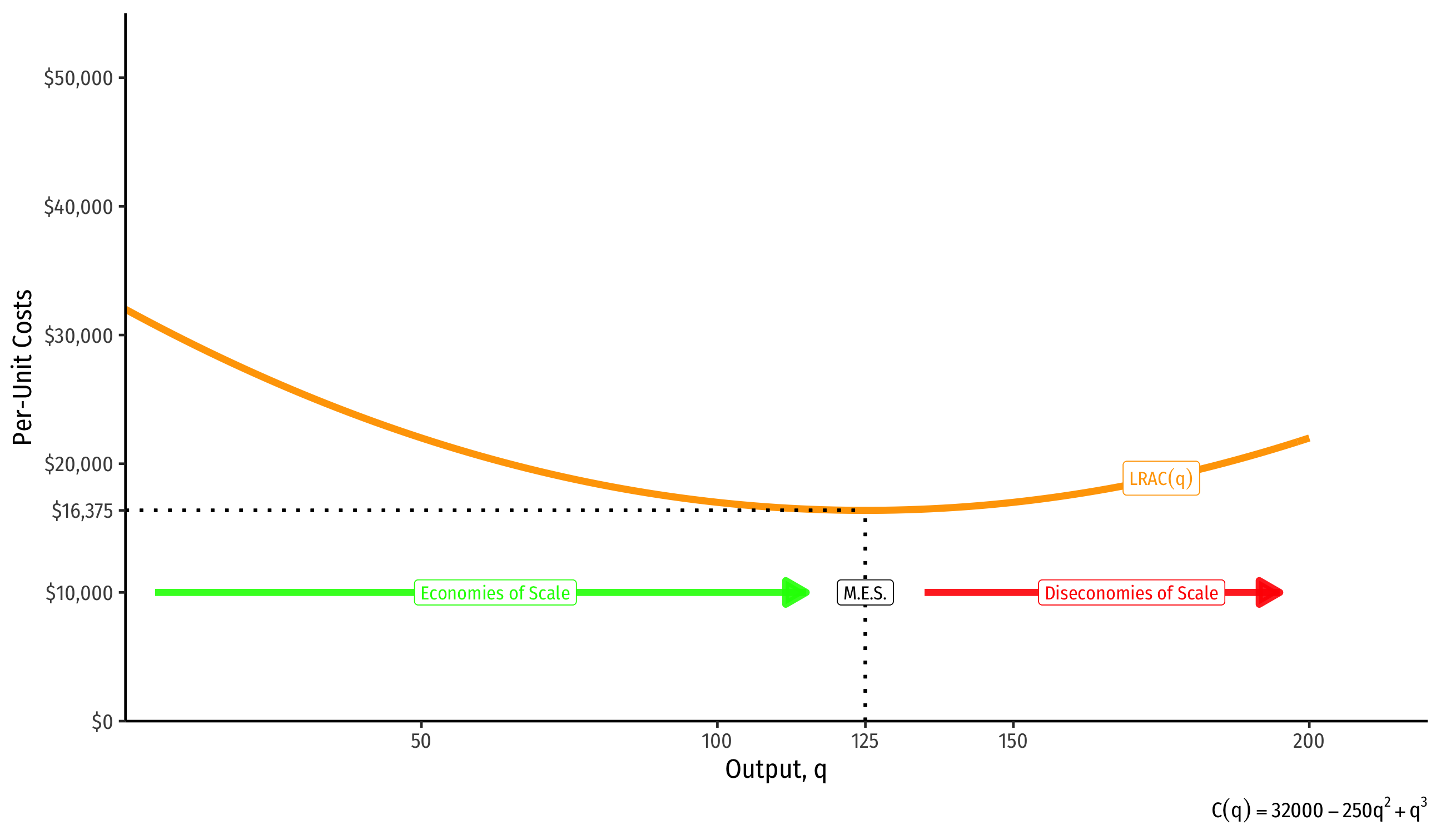
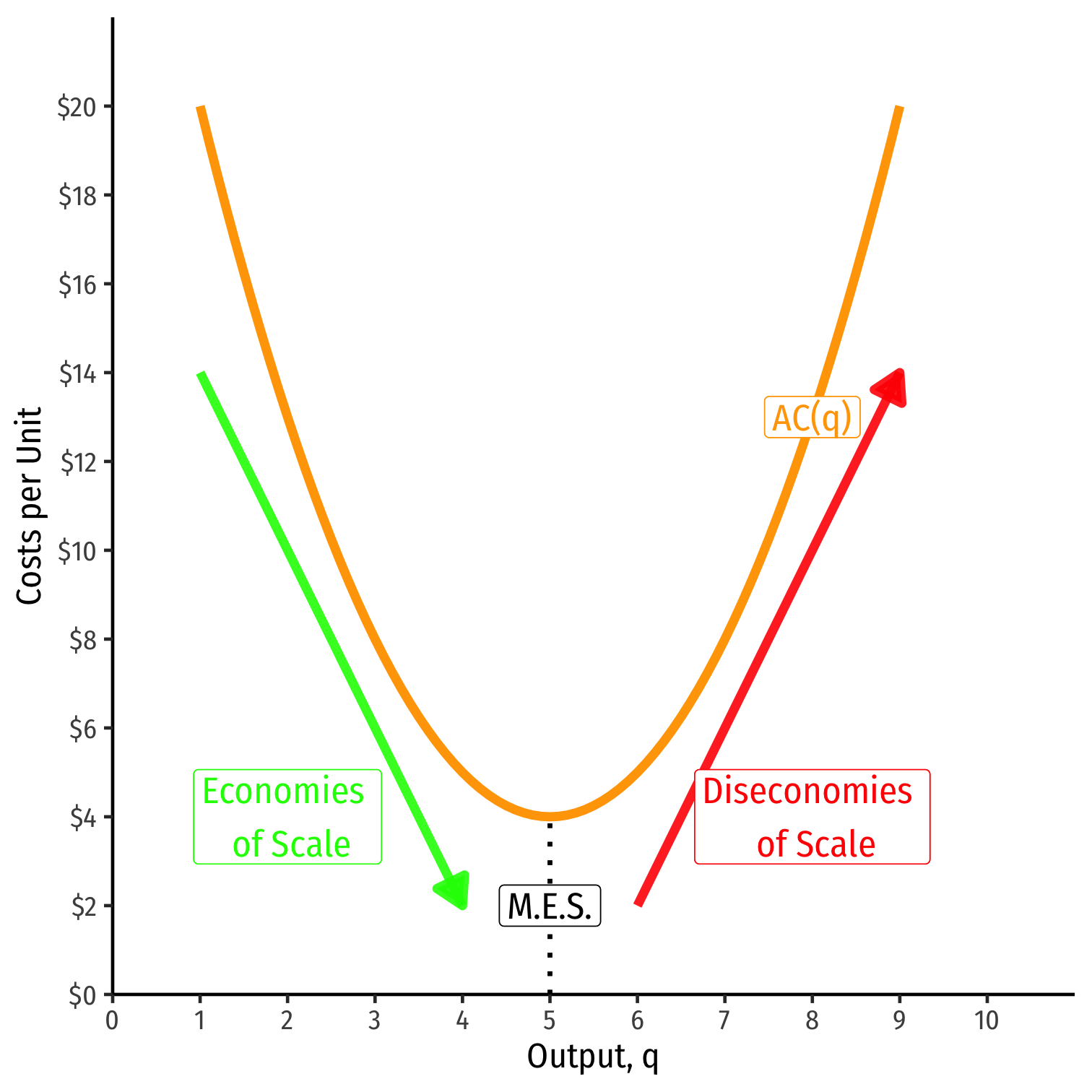
Long Run Costs & Scale Economies II
Minimum Efficient Scale: q with the lowest AC(q)
Economies of Scale: ↑q, ↓AC(q)
Diseconomies of Scale: ↑q, ↑AC(q)
Long Run Costs and Scale Economies: Example