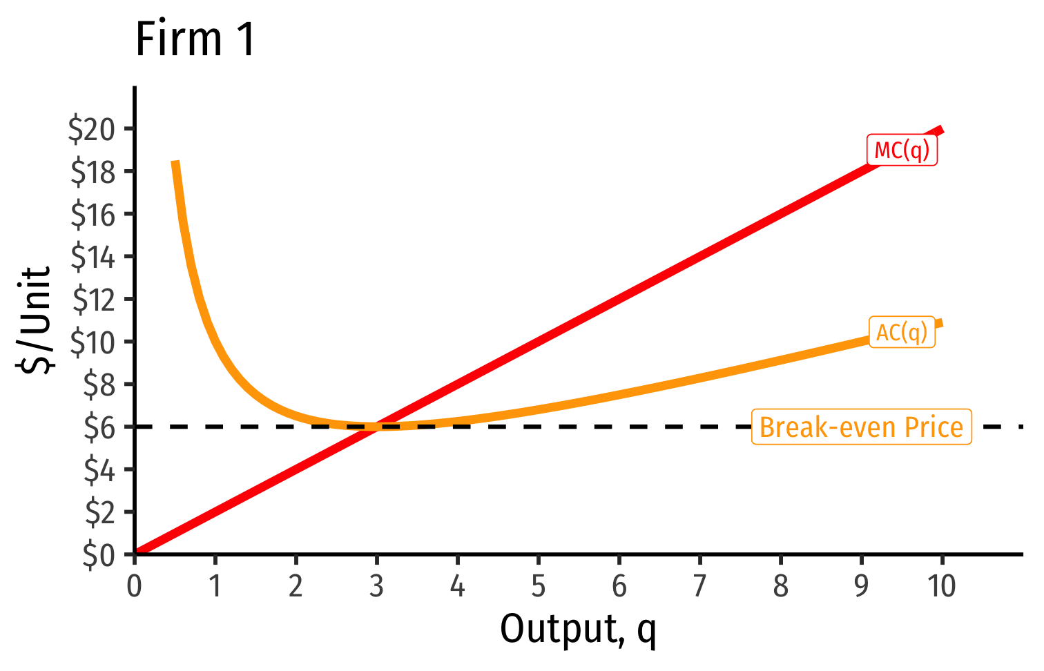
Firm Decisions in the Long Run I
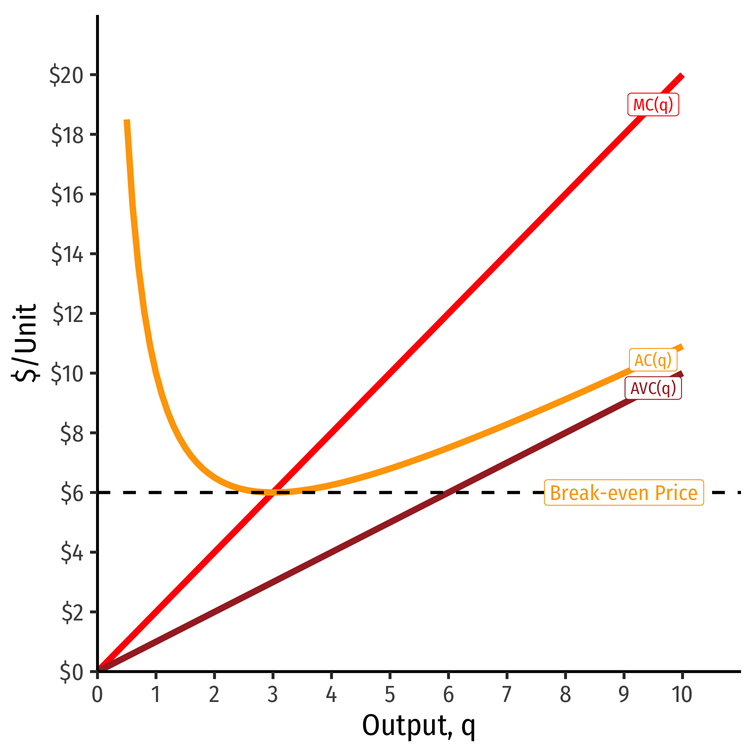
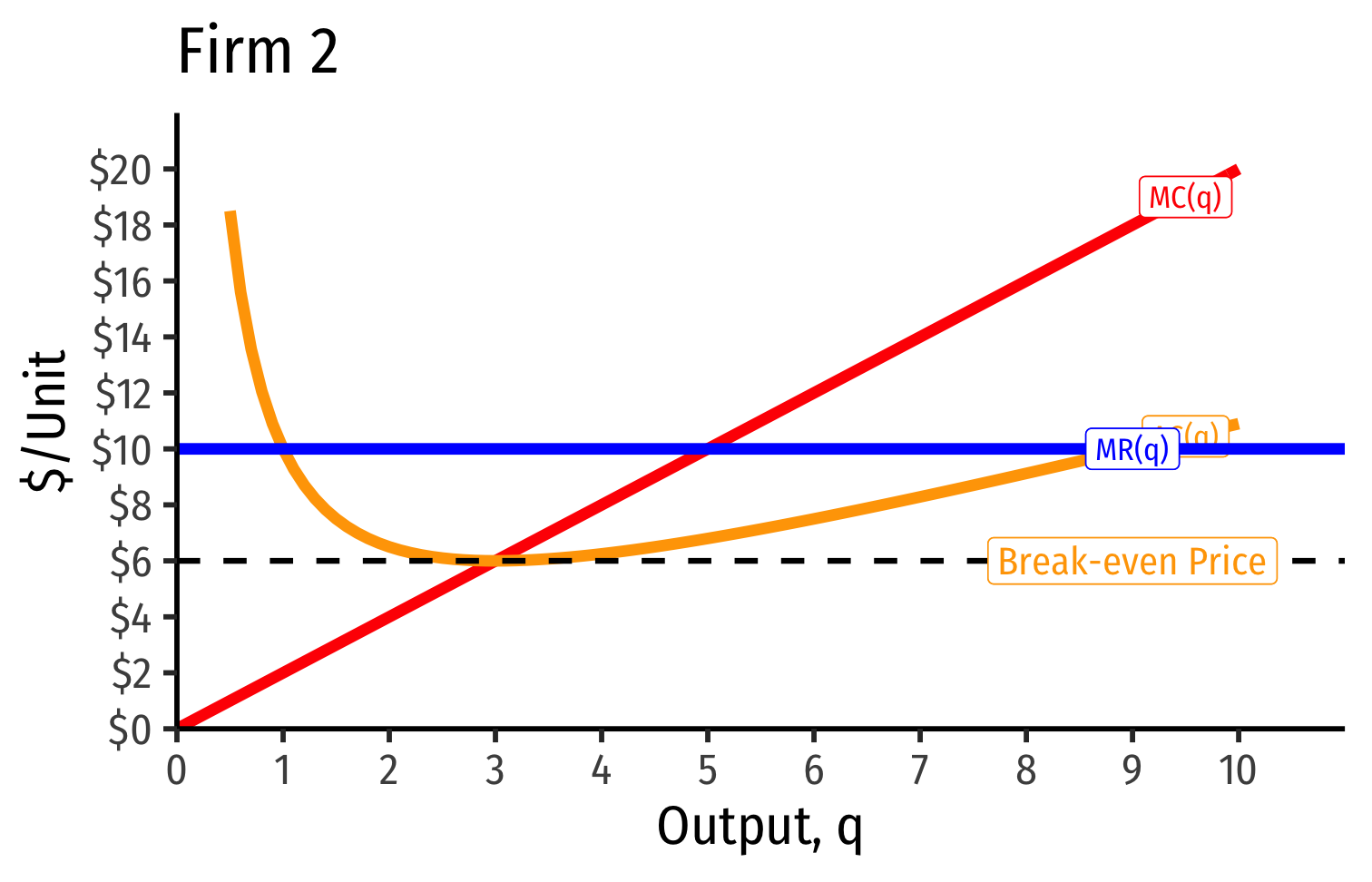
AC(q)min at a market price of $6
- Firm earns “normal” economic profits (of 0)
At any market price below $6.00, firm earns losses
- Short Run: firm shuts down if p<AVC(q)
At any market price above $6.00, firm earns “supernormal” profits (>0)
Firm Supply Decisions in the Short Run vs. Long Run
Short run: firms that shut down (q∗=0) stuck in market, incur fixed costs π=−f
Long run: firms earning losses (π<0) can exit the market and earn π=0
- No more fixed costs, firms can sell/abandon f at q∗=0
Firm Supply Decisions in the Short Run vs. Long Run
Short run: firms that shut down (q∗=0) stuck in market, incur fixed costs π=−f
Long run: firms earning losses (π<0) can exit the market and earn π=0
- No more fixed costs, firms can sell/abandon f at q∗=0
Entrepreneurs not currently in market can enter and produce, if entry would earn them π>0

Firm Supply Decisions in the Short Run vs. Long Run

Firm Supply Decisions in the Short Run vs. Long Run

Firm's Long Run Supply: Visualizing
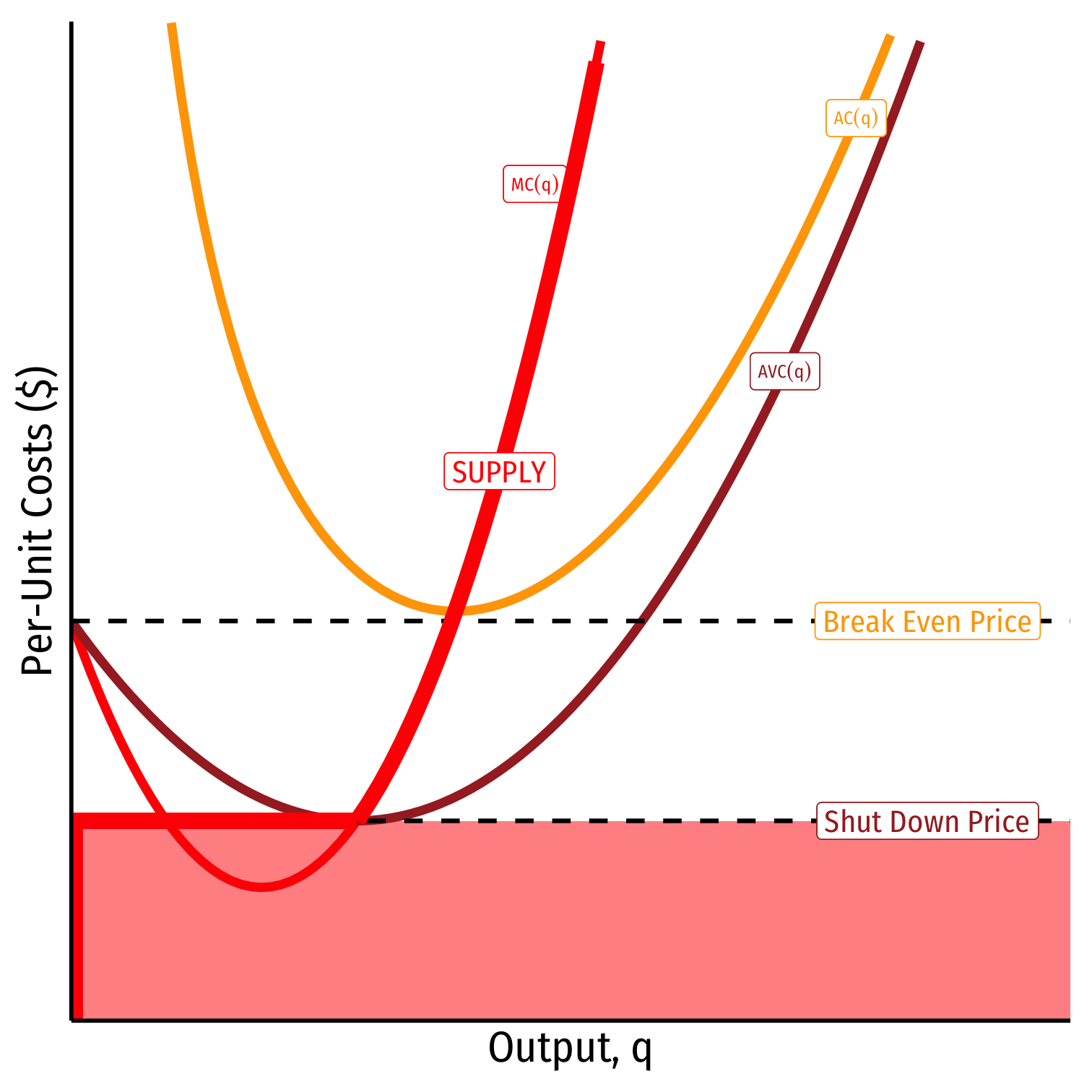
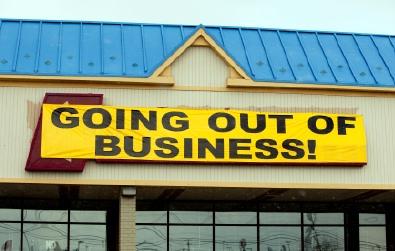
When p<AVC
Profits are negative
Short run: shut down production
- Firm loses more π by producing than by not producing
Long run: firms in industry exit the industry
- No new firms will enter this industry
Firm's Long Run Supply: Visualizing
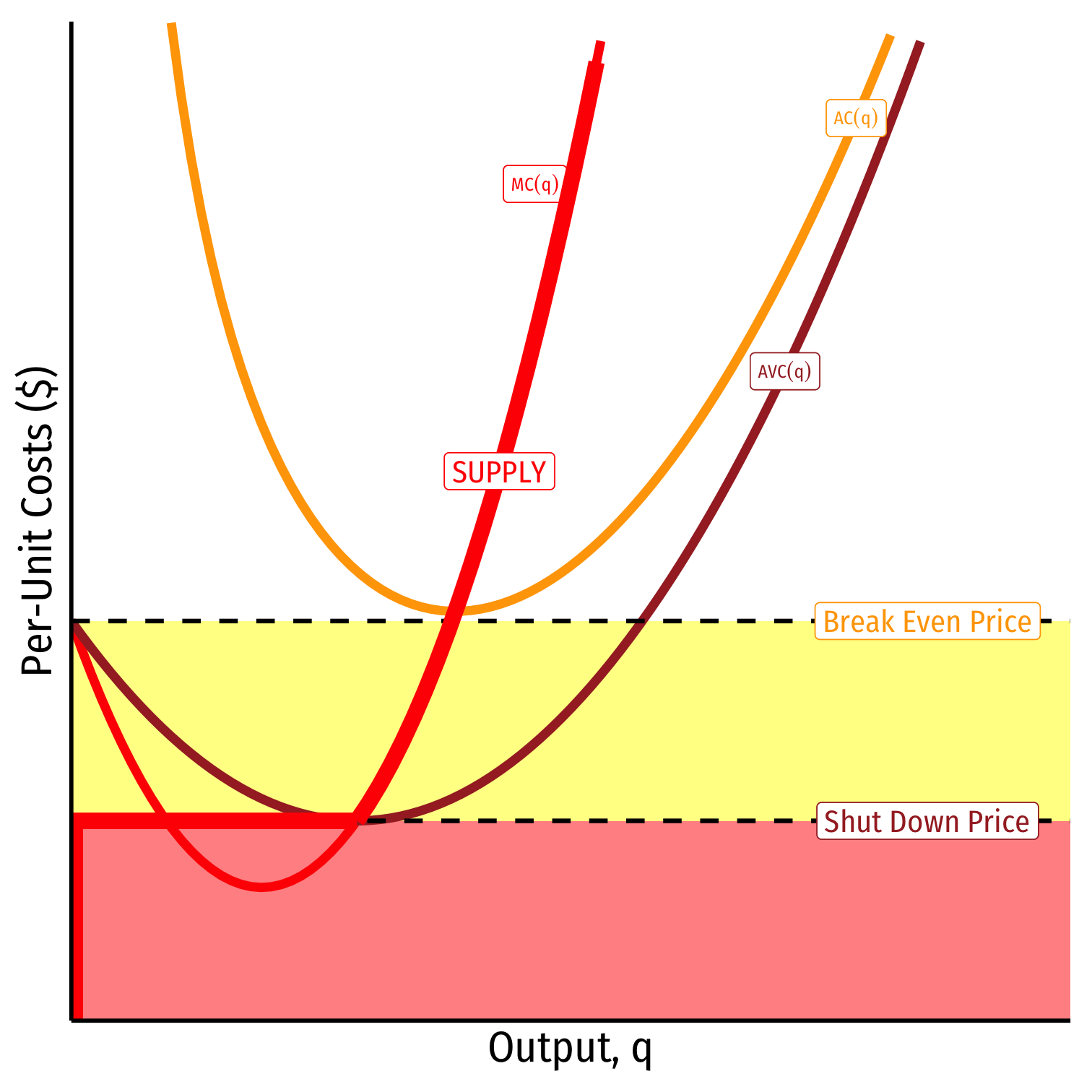
When AVC<p<AC
Profits are negative
Short run: continue production
- Firm loses less π by producing than by not producing
Long run: firms in industry exit the industry
- No new firms will enter this industry
Firm's Long Run Supply: Visualizing
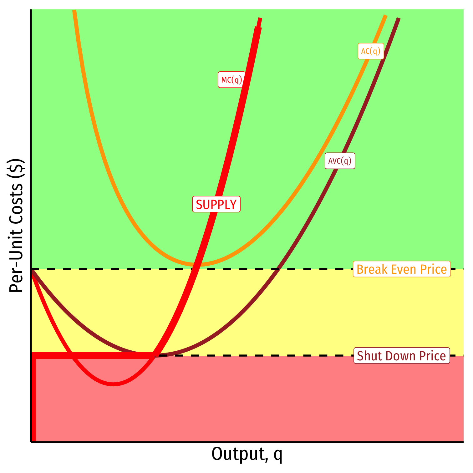
When AC<p
Profits are positive
Short run: continue production
- Firm earning profits
Long run: firms in industry stay in industry
- New firms will enter this industry
Exit, Entry, and Long Run Industry Equilibrium I
Now we must combine optimizing individual firms with market-wide adjustment to equilibrium
Since π=[p−AC(q)]q, in the long run, profit-seeking firms will:
- Enter markets where p>AC(q)
Exit, Entry, and Long Run Industry Equilibrium I
Now we must combine optimizing individual firms with market-wide adjustment to equilibrium
Since π=[p−AC(q)]q, in the long run, profit-seeking firms will:
- Enter markets where p>AC(q)
- Exit markets where p<AC(q)
Exit, Entry, and Long Run Industry Equilibrium II
- Long-run equilibrium: entry and exit ceases when p=AC(q) for all firms, implying normal economic profits of π=0
Exit, Entry, and Long Run Industry Equilibrium II
Long-run equilibrium: entry and exit ceases when p=AC(q) for all firms, implying normal economic profits of π=0
Zero Economic Profits Theorem: long run economic profits for all firms in a competitive industry are 0
Firms must earn an accounting profit to stay in business
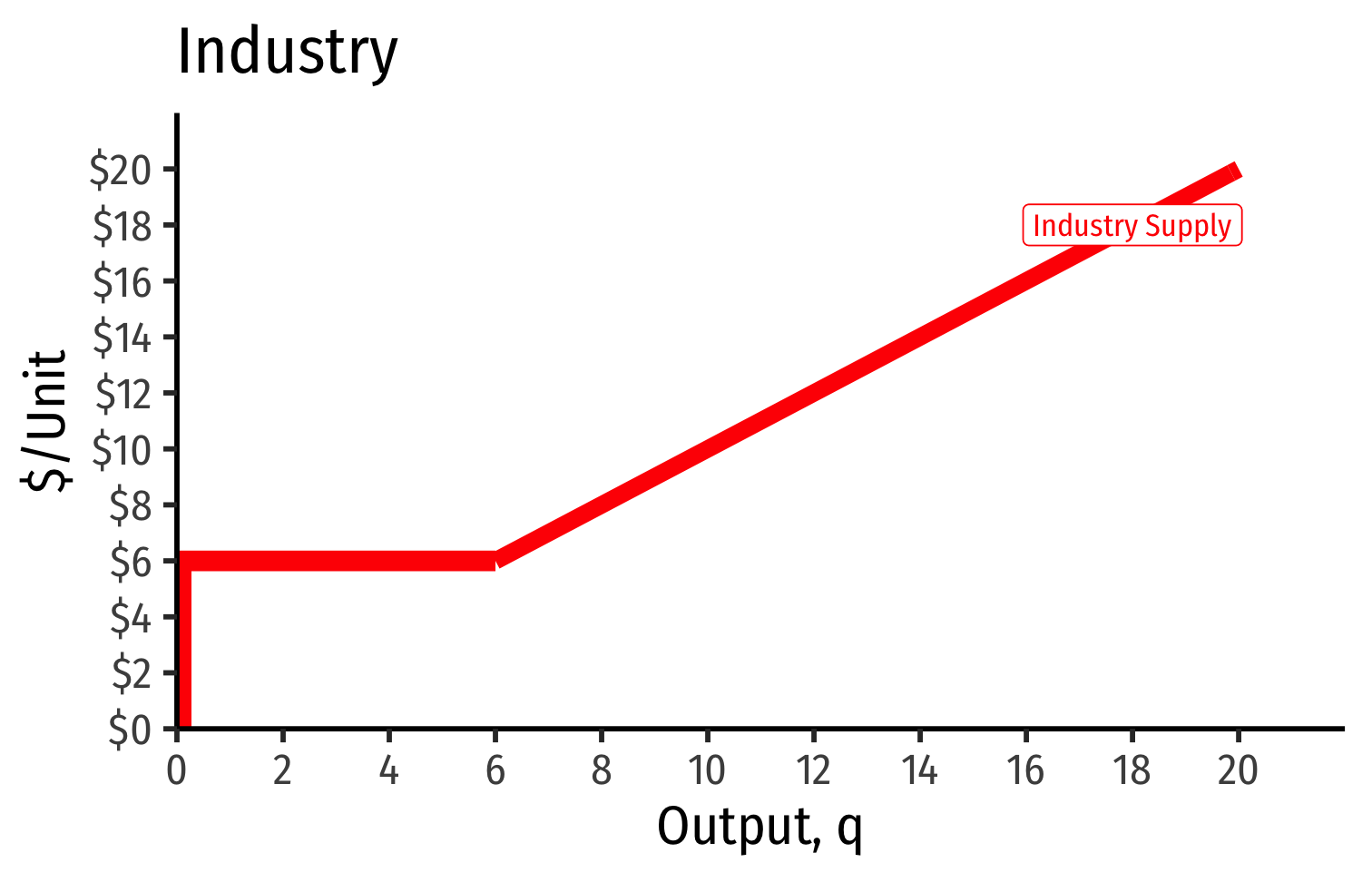
Industry Supply Curves (Identical Firms)

Industry Supply Curves (Identical Firms)
- Industry supply curve is the horizontal sum of all individual firm's supply curves
- Which are each firm's marginal cost curve above its breakeven price
Industry Supply Curves (Identical Firms)

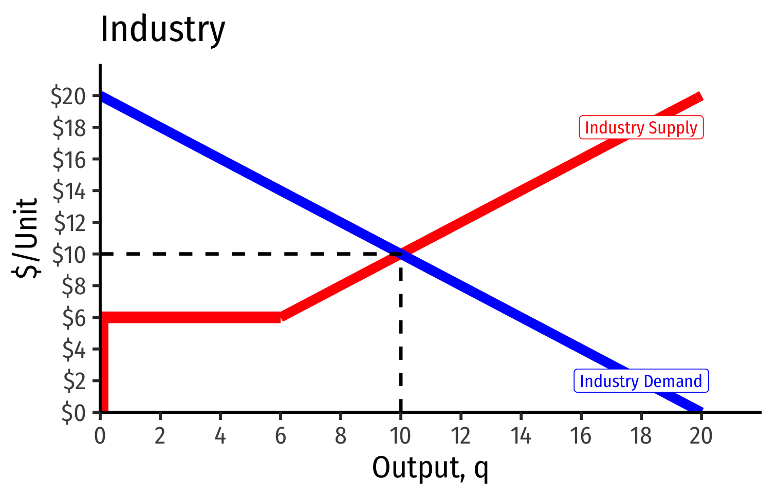
- Industry demand curve (where equal to supply) sets market price, demand for firms
Industry Supply Curves (Identical Firms)

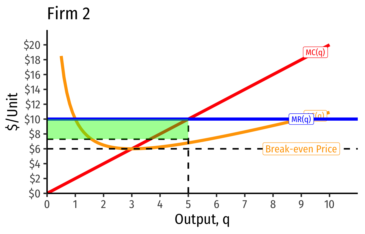

Short Run: each firm is earning profits p>AC(q)
Long run: induces entry by firm 3, firm 4, ⋯, firm n
Industry Supply Curves (Identical Firms)
Short Run: each firm is earning profits p>AC(q)
Long run: induces entry by firm 3, firm 4, ⋯, firm n
- Long run industry equilibrium:
Industry Supply Curves (Identical Firms)
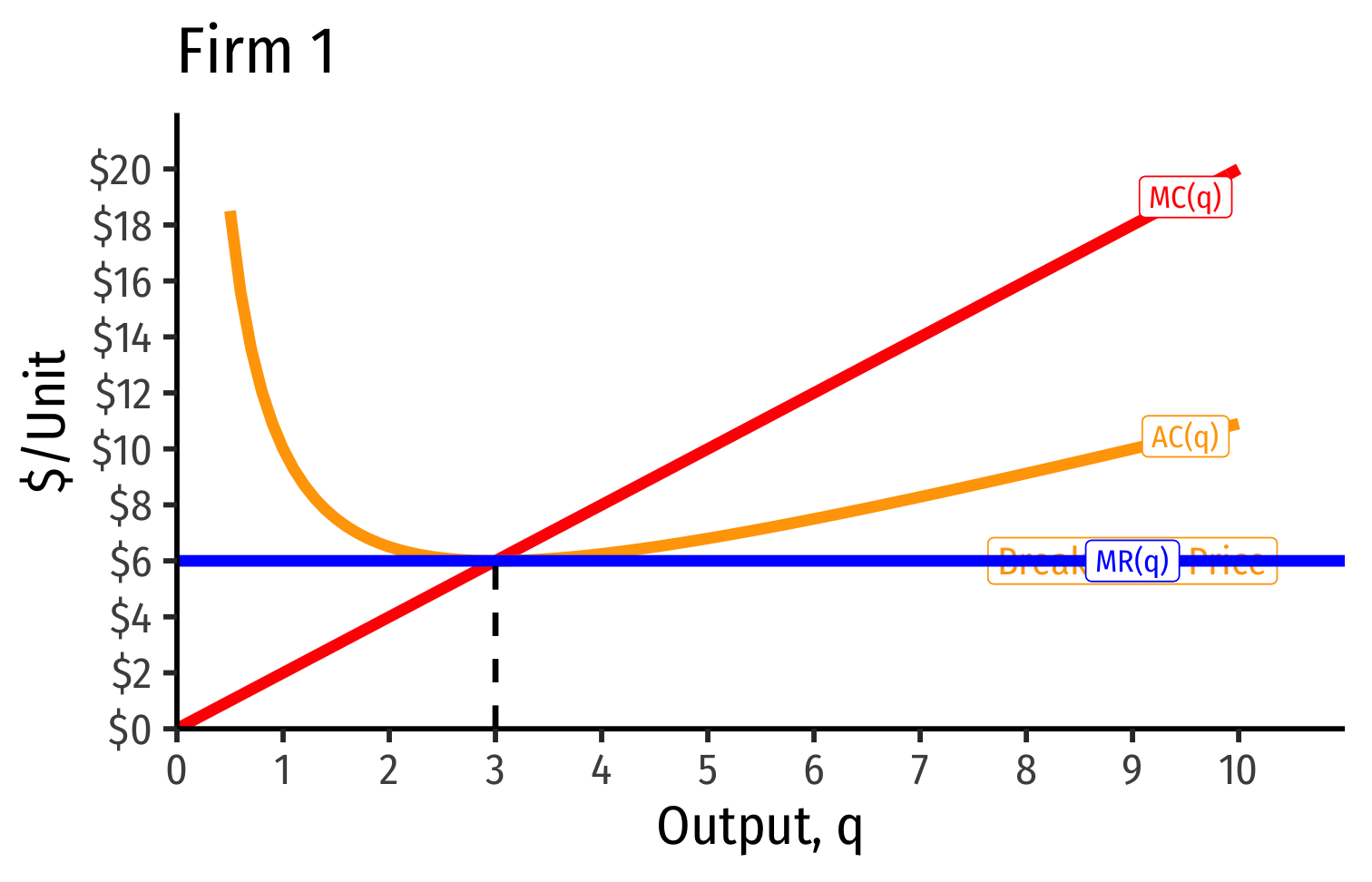
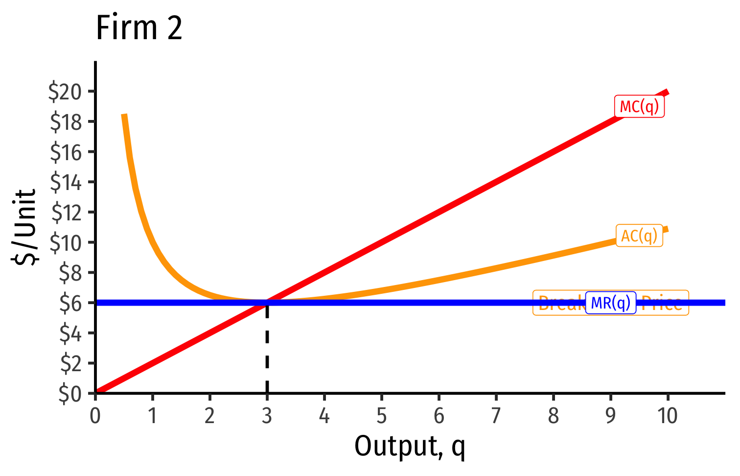
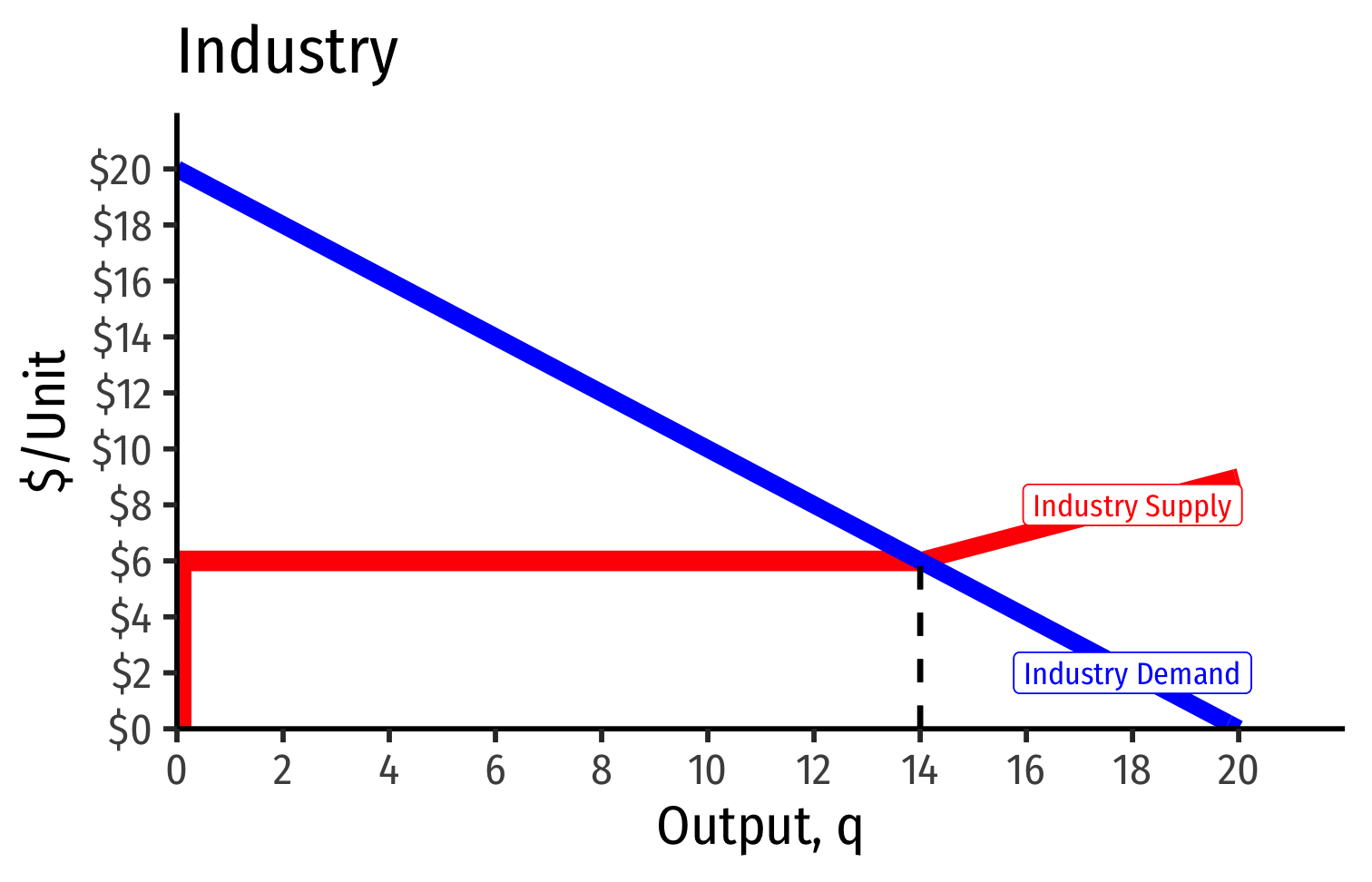
Short Run: each firm is earning profits p>AC(q)
Long run: induces entry by firm 3, firm 4, ⋯, firm n
Long run industry equilibrium: p=AC(q)min, π=0 at p= $6; supply becomes more elastic
Back to Zero Economic Profits
- Recall, we've essentially defined a firm as a completely replicable recipe (production function) of resources
q=f(L,K)
- “Any idiot” can enter market, buy required (L,K) at prices (w,r), produce q∗ at market price p and earn the market rate of π
Back to Zero Economic Profits
Zero long run economic profit ≠ industry disappears, just stops growing
Less attractive to entrepreneurs & start ups to enter than other, more profitable industries
These are mature industries (again, often commodities), the backbone of the economy, just not sexy!

Back to Zero Economic Profits
All factors being paid their market price
- i.e. their opportunity cost — what they could earn elsewhere in economy
Firms earning normal market rate of return
- No excess rewards (economic profits) to attract new resources into the industry, nor losses to bleed resources out of industry
Back to Zero Economic Profits
But we've so far been imagining a market where every firm is identical, just a recipe “any idiot” can copy
What about if firms have different technologies or costs?
Industry Supply Curves (Different Firms) I
Firms have different technologies/costs due to relative differences in:
- Managerial talent
- Worker talent
- Location
- First-mover advantage
- Technological secrets/IP
- License/permit access
- Political connections
- Lobbying
Let's derive industry supply curve again, and see how this may affect profits

Industry Supply Curves (Different Firms) II
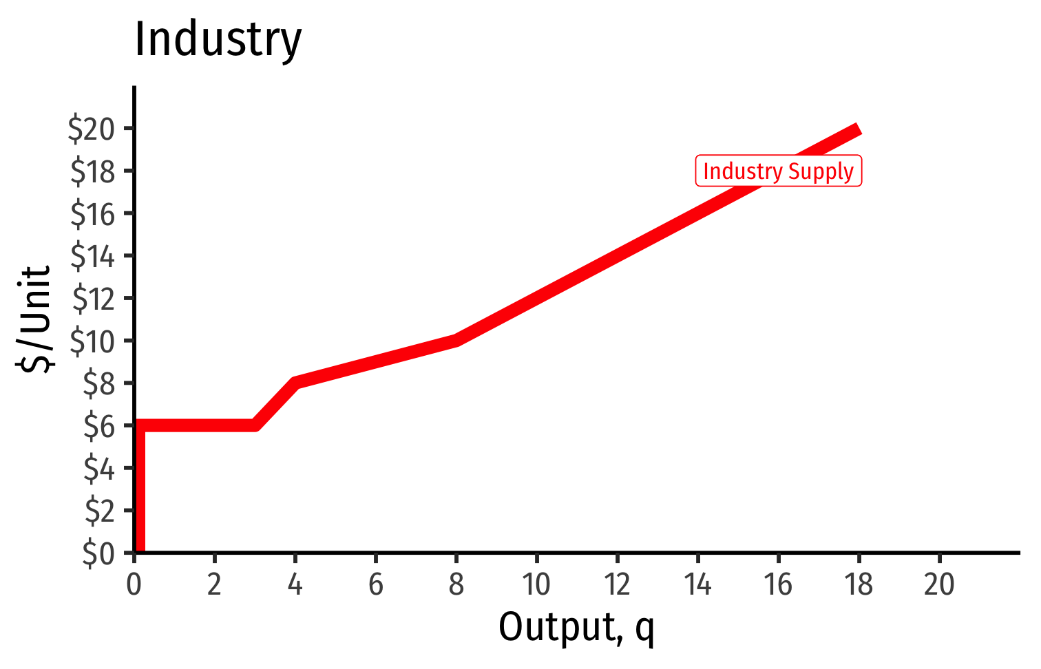
Industry Supply Curves (Different Firms) II
- Industry supply curve is the horizontal sum of all individual firm's supply curves
- Which are each firm's marginal cost curve above its breakeven price
Industry Supply Curves (Different Firms) II

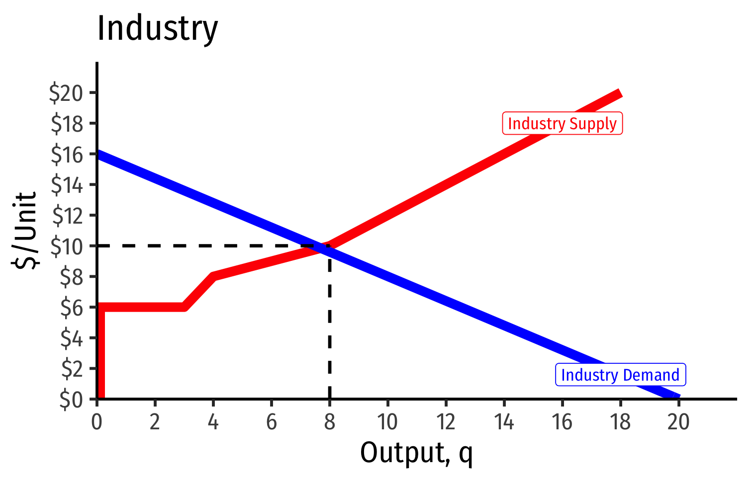
Industry Supply Curves (Different Firms) II
- Industry demand curve (where equal to supply) sets market price, demand for firms
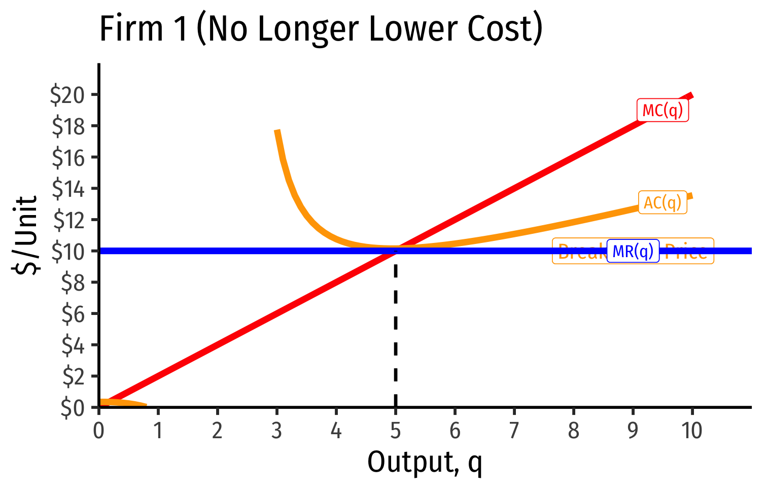
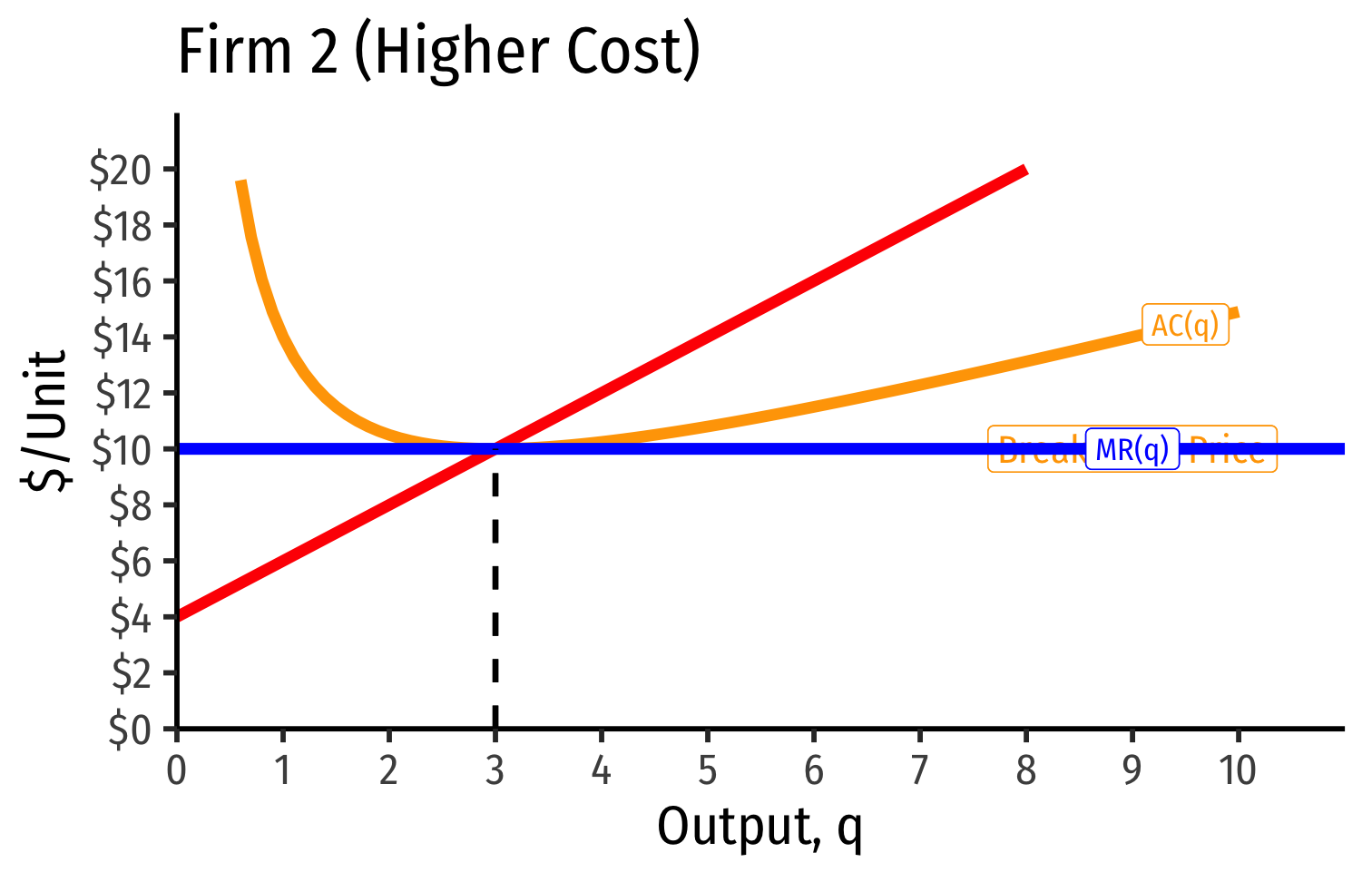
Industry Supply Curves (Different Firms) II
- Industry demand curve (where equal to supply) sets market price, demand for firms
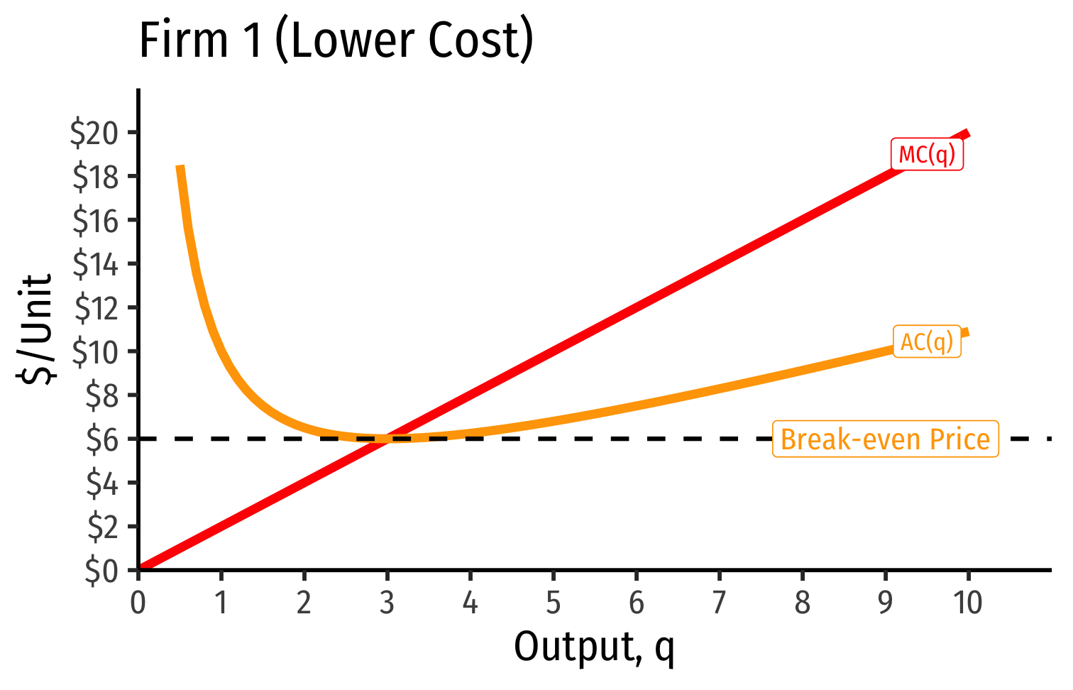
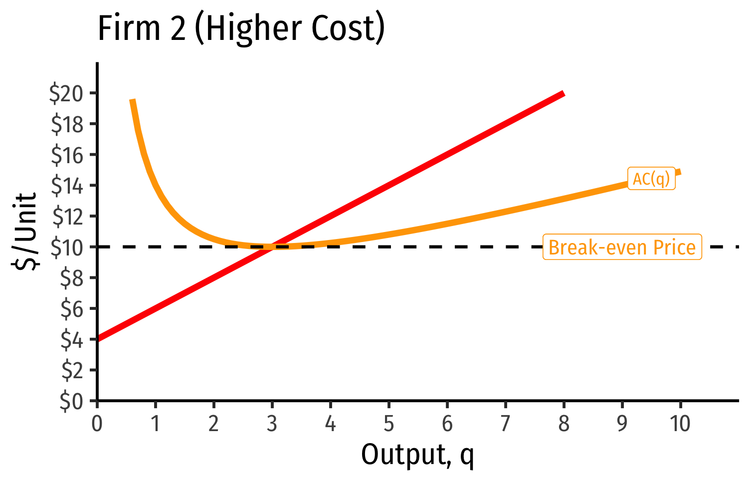
- Long run industry equilibrium: p=AC(q)min, π=0 for marginal (highest cost) firm (Firm 2)
Industry Supply Curves (Different Firms) II
- Industry demand curve (where equal to supply) sets market price, demand for firms
- Long run industry equilibrium: p=AC(q)min, π=0 for marginal (highest cost) firm (Firm 2)
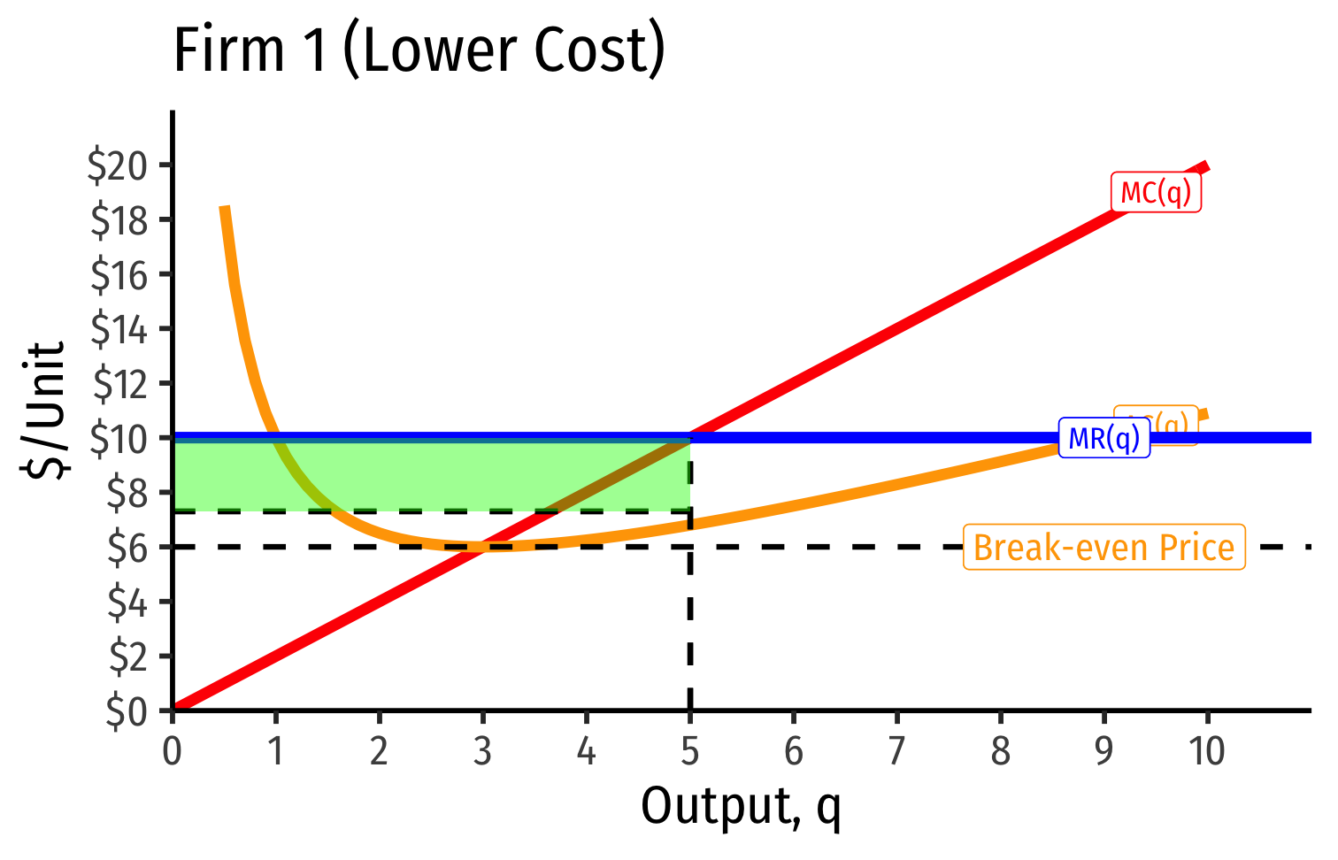
- Firm 1 (lower cost) appears to be earning profits...(we’ll come back to this)
Economic Rents and Zero Economic Profits I

- With differences between firms, long-run equilibrium p=AC(q)min of the marginal (highest-cost) firm
- If p>AC(q) for that firm, would induce more entry into industry!
Economic Rents and Zero Economic Profits I
“Inframarginal” (lower-cost) firms earn economic rents
- returns higher than their opportunity cost (what is needed to bring them into this industry)
Economic rents arise from relative differences between firms
- actually using different inputs!
Economic Rents and Zero Economic Profits III
Some factors are relatively scarce in the whole economy
- (talent, location, secrets, IP, licenses, being first, political favoritism)
Inframarginal firms that use these scarce factors gain an advantage
It would seem these firms earn profits (like Firm 1), as they have lower costs...
- ...But what will happen to the prices for their scarce factors over time?
Economic Rents and Zero Economic Profits IV

Rival firms willing to pay for rent-generating factor to gain advantage
Competition over acquiring the scarce factors pushes up their prices
- i.e. costs to firms of using the factor!
Rents are included in the opportunity cost (price) for inputs over long run
- Must pay a factor enough to keep it out of other uses
Economic Rents and Zero Economic Profits V
Economic rents ≠ economic profits!
- Rents actually reduce profits!
Firm does not earn the rents, they raise firm's costs and squeeze out profits!
Owners of scarce factors (workers, landowners, inventors, etc) earn the rents as higher income for their services (wages, rents, interest, royalties, etc).
Economic Rents Reduce Profits


- Short Run: firm that possesses scarce rent-generating factors has lower costs, perhaps short-run profits
Economic Rents Reduce Profits
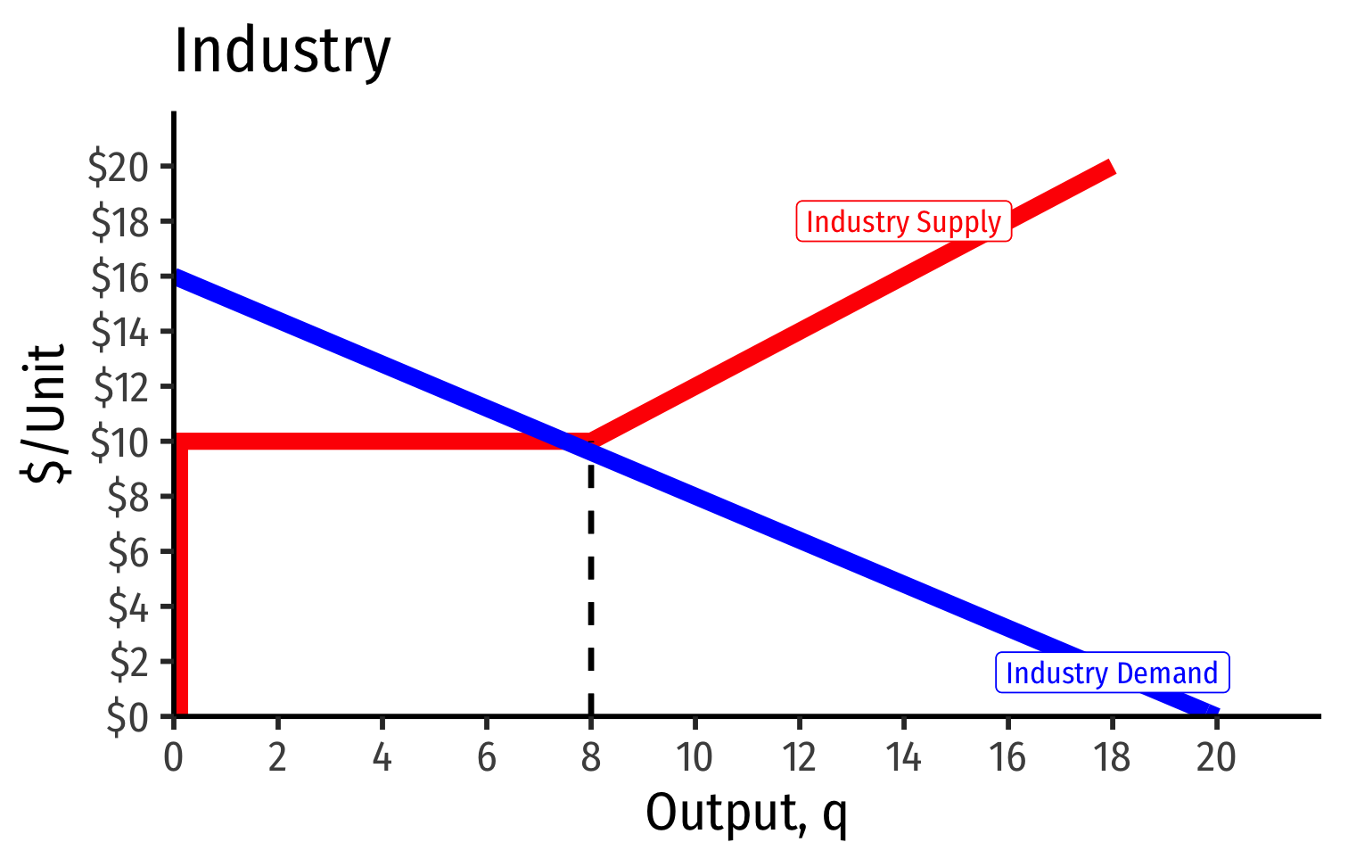
Short Run: firm that possesses scarce rent-generating factors has lower costs, perhaps short-run profits
Long run: competition over those factors pushes up their prices, raising costs to firm, until its profits go to zero as well
- Increase in fixed cost (scarce factor), raising AC(q), which now includes rents (more info here)
Recall: Accounting vs. Economic Point of View
Recall “economic point of view”:
Producing your product pulls scarce resources out of other productive uses in the economy
Profits attract resources: pulled out of other (less valuable) uses
Losses repel resources: pulled away to other (more valuable) uses
Zero profits keep resources where they are
- Implies society is using resources optimally


Supply Function
- Supply function relates quantity to price
Example: q=2p−4
- Not graphable (wrong axes)!

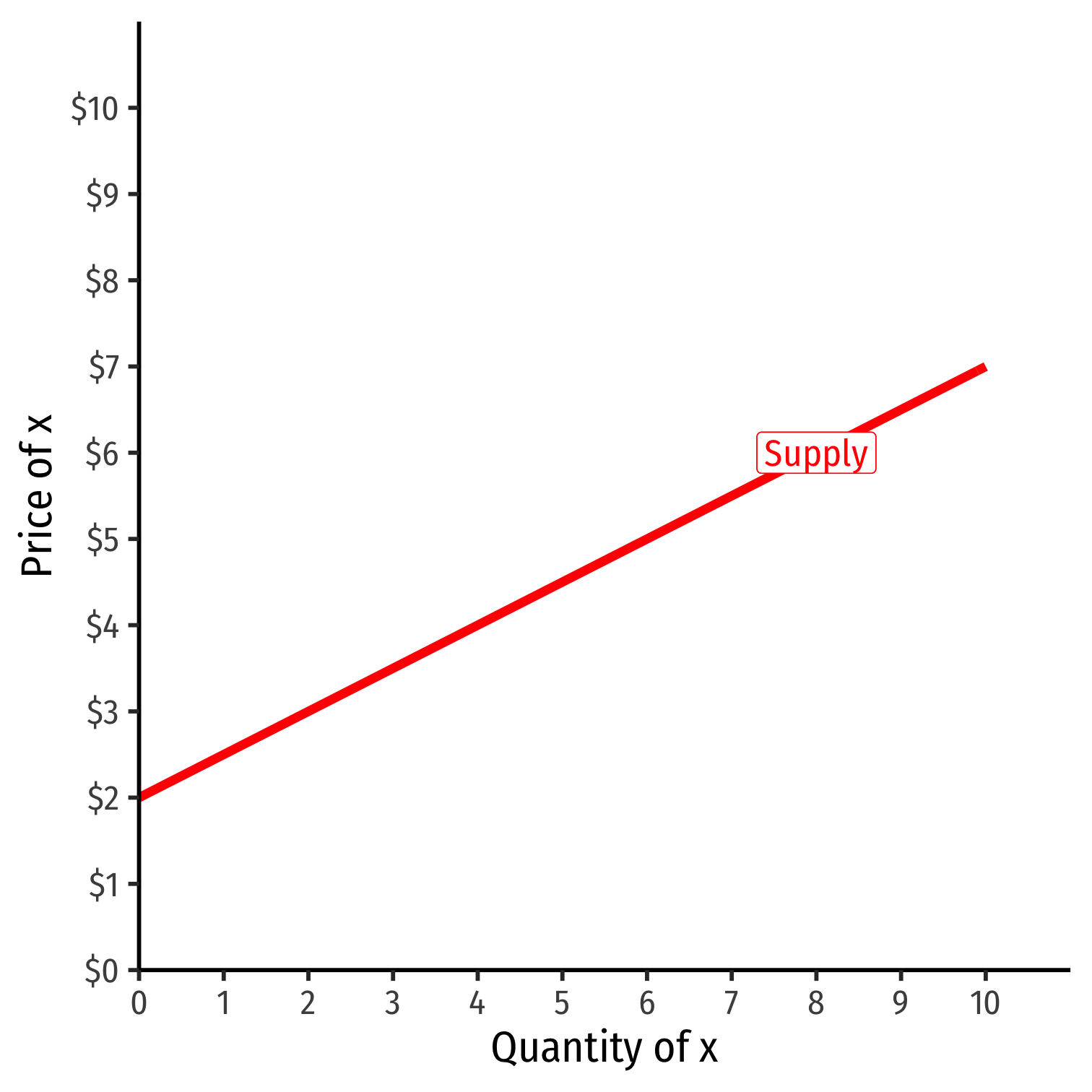
Inverse Supply Function
- Inverse supply function relates price to quantity
- Take supply function, solve for p
Example: p=2+0.5q
- Graphable (price on vertical axis)!
Inverse Supply Function
Example: p=2+0.5q
Slope: 0.5
Vertical intercept called the "Choke price": price where qS=0 ($2), just low enough to discourage any sales

Inverse Supply Function
Read two ways:
Horizontally: at any given price, how many units firm wants to sell
Vertically: at any given quantity, the minimum willingness to accept (WTA) for that quantity

Price Elasticity of Supply
- Price elasticity of supply measures how much (in %) quantity supplied changes in response to a (1%) change in price
ϵqS,p=%ΔqS%Δp

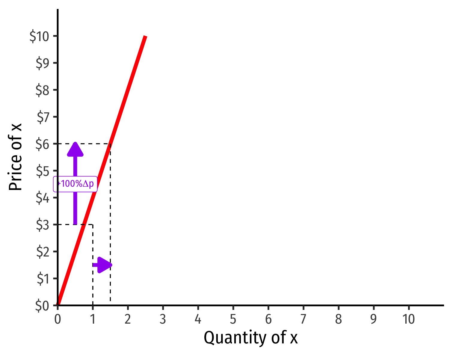
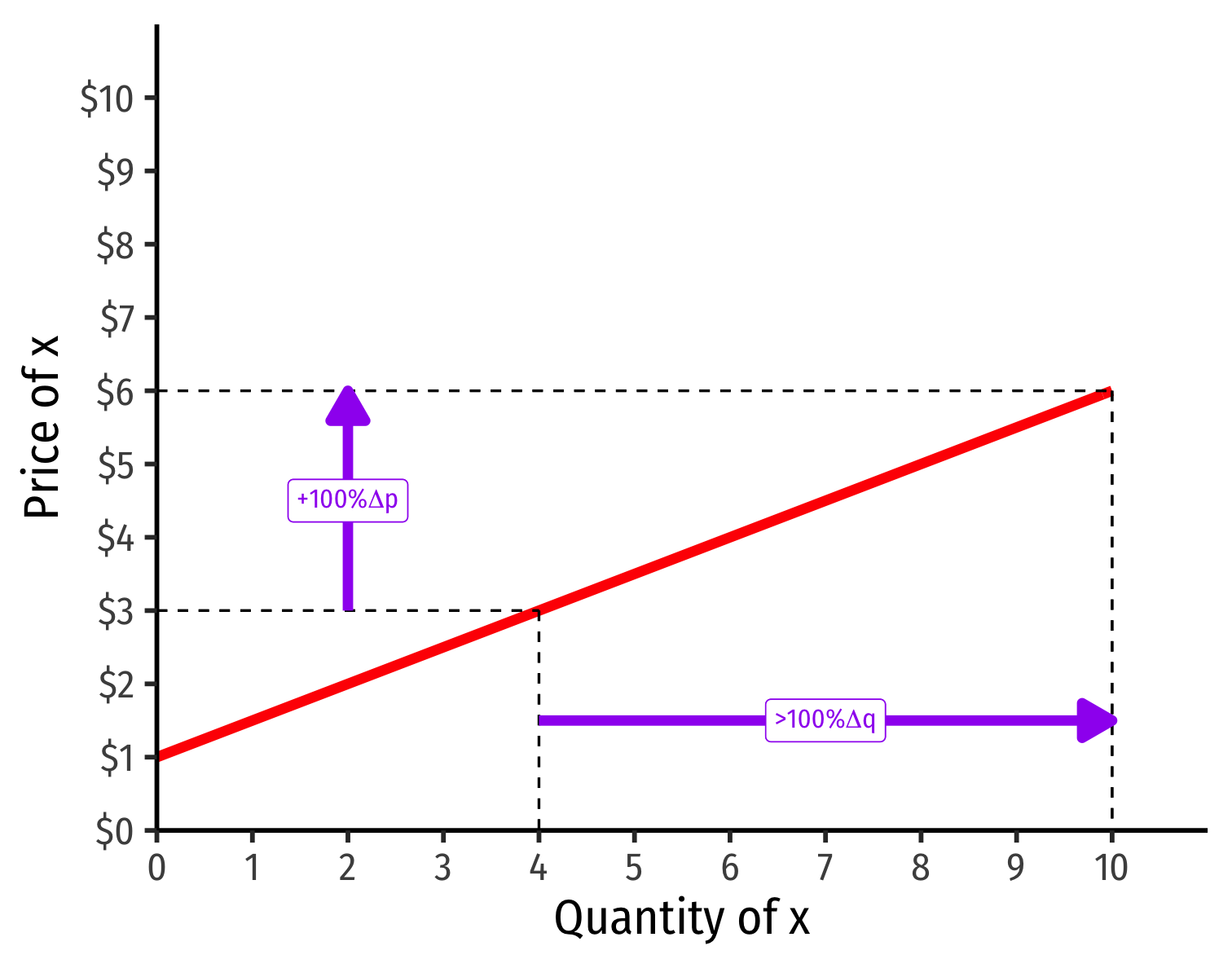
Visualizing Price Elasticity of Supply
An identical 100% price increase on an:
"Inelastic" Supply Curve
"Elastic" Supply Curve
Price Elasticity of Supply Formula
ϵq,p=1slope×pq
First term is the inverse of the slope of the inverse supply curve (that we graph)!
To find the elasticity at any point, we need 3 things:
- The price
- The associated quantity supplied
- The slope of the (inverse) supply curve
Price Elasticity of Supply Changes Along the Curve
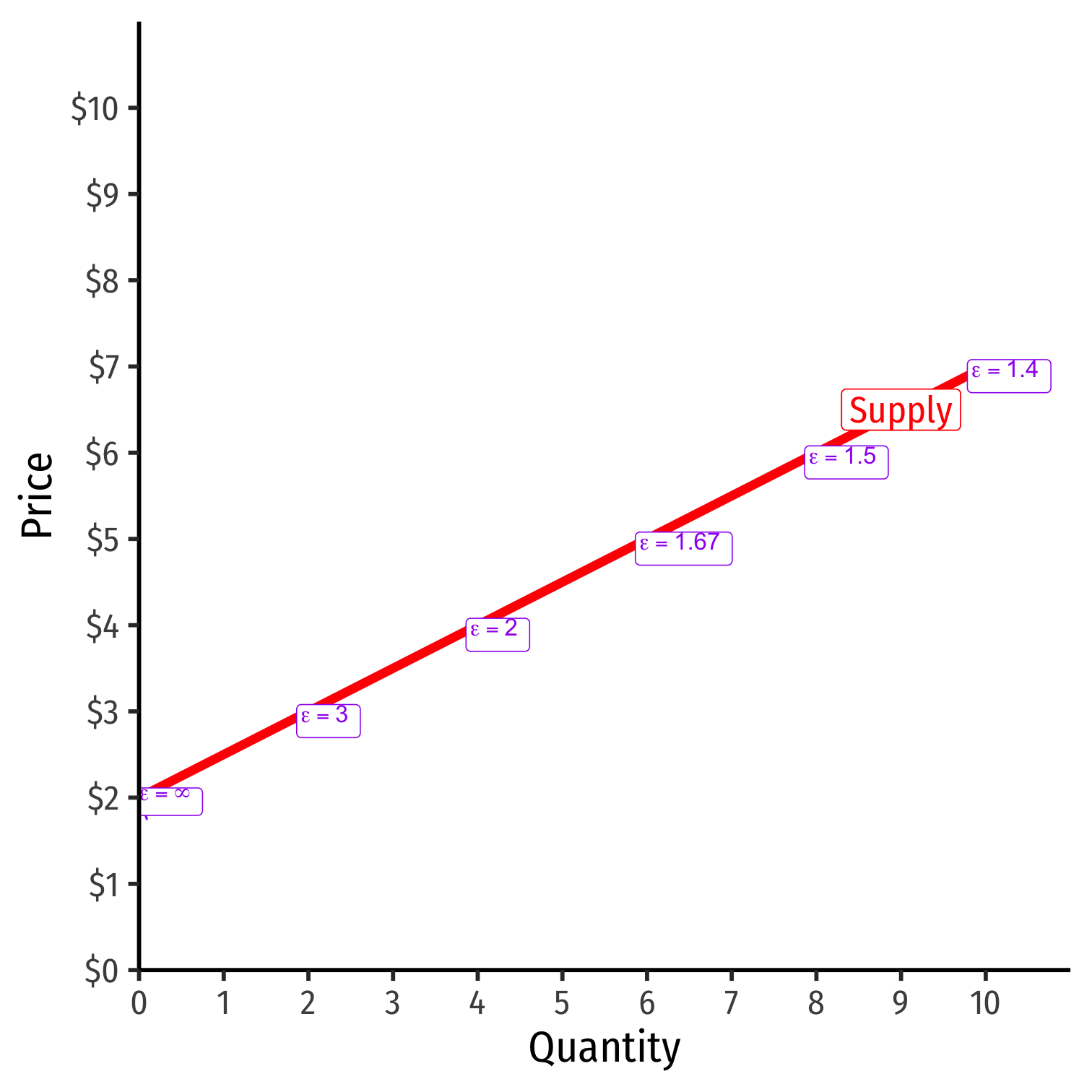
ϵq,p=1slope×pq
Elasticity ≠ slope (but they are related)!
Elasticity changes along the supply curve
Often gets less elastic as ↑ price (↑ quantity)
- Harder to supply more
Determinants of Price Elasticity of Supply I
What determines how responsive your selling behavior is to a price change?
The faster (slower) costs increase with output ⟹ less (more) elastic supply
- Mining for natural resources vs. automated manufacturing
Smaller (larger) share of market for inputs ⟹ more (less) elastic
- Will your suppliers raise the price much if you buy more?
- How much competition is there in your input markets?
Determinants of Price Elasticity of Supply II
What determines how responsive your selling behavior is to a price change?
- More (less) time to adjust to price changes ⟹ more (less) elastic
- Supply of oil today vs. oil in 10 years
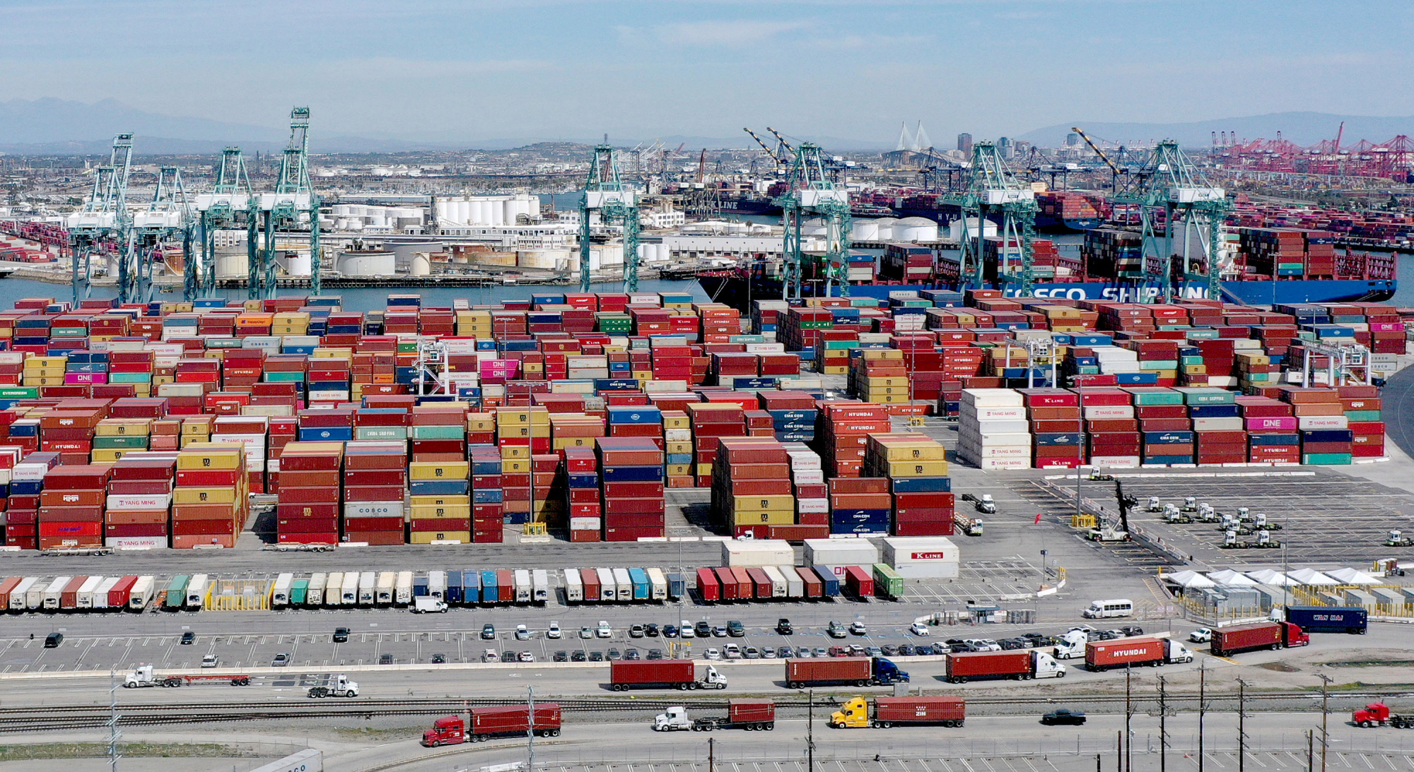
Price Elasticity of Supply: Examples
Price Elasticity of Supply: Examples

Price Elasticity of Supply: Examples
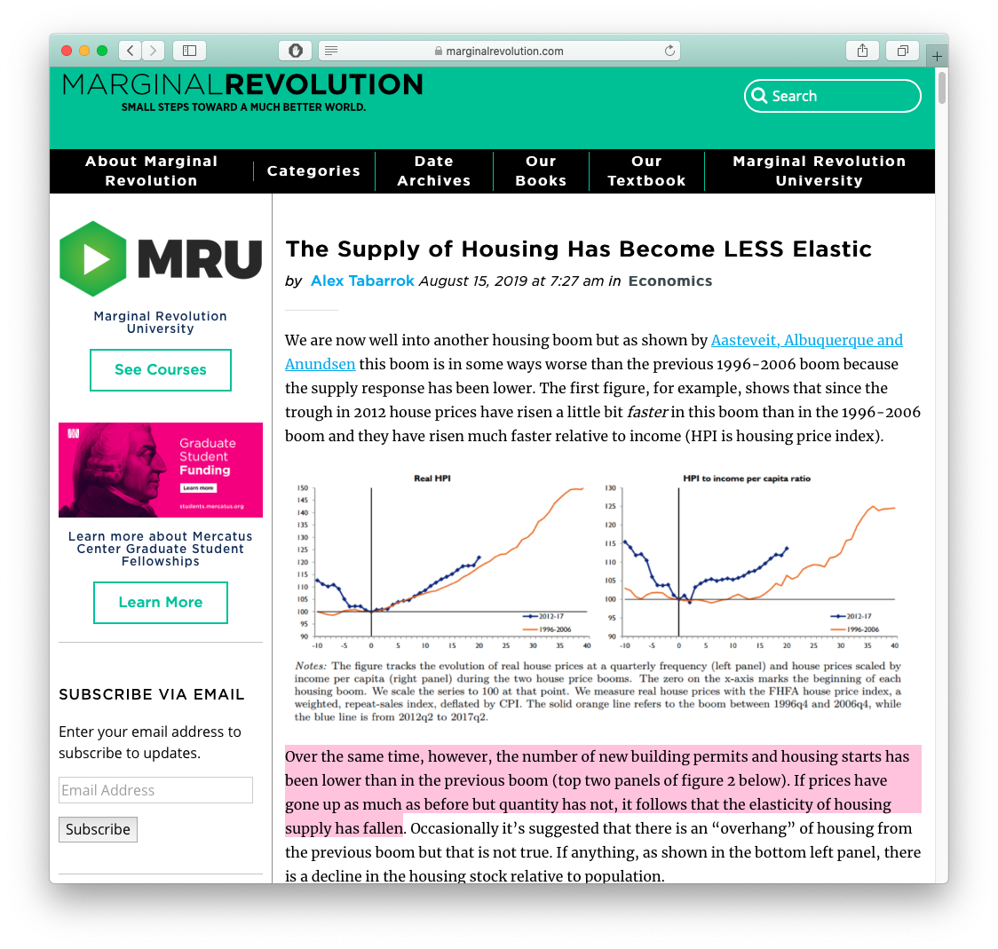
“[T]he number of new building permits and housing starts has been lower than in the previous boom...if prices have gone up as much as before but quantity has not, it follows that the elasticity of supply has fallen.”
Price Elasticity of Supply: Examples

Source: Washington Post (Oct 2, 2021): “Inside America’s Broken Supply Chain”
Price Elasticity of Supply: Examples